
Transformation of the Beta Distribution for Color Transfer
Hristina Hristova, Olivier Le Meur, R
´
emi Cozot and Kadi Bouatouch
University of Rennes 1, 263 Avenue G
´
en
´
eral Leclerc, 35000 Rennes, France
Keywords:
Beta Distribution, Bounded Distributions, Color Transfer, Transformation of Bounded Distributions.
Abstract:
In this paper, we propose a novel transformation between two Beta distributions. Our transformation progres-
sively and accurately reshapes an input Beta distribution into a target Beta distribution using four intermediate
statistical transformations. The key idea of this paper is to adopt the Beta distribution to model the discrete
distributions of color and light in images. We design a new Beta transformation which we apply in the context
of color transfer between images. Experiments have shown that our method obtains more natural and less
saturated results than results of recent state-of-the-art color transfer methods. Moreover, our results portray
better both the target color palette and the target contrast.
1 INTRODUCTION
The Gaussian distribution is a well-known and well-
studied continuous unbounded distribution with many
applications to image processing. The Gaussian
distribution is commonly adopted to fit the distri-
butions of various image features, such as color
and light (Reinhard et al., 2001). The analyti-
cally tractable function and relative simplicity of
the Gaussian distribution reveal its significance to
problems like transportation optimization (Olkin and
Pukelsheim, 1982), color correction for image mo-
saicking (Oliveira et al., 2011), example-based color
transfer (Faridul et al., 2014), etc.
Color transfer between images has raised a lot
of interest during the past decade. Color transfer
transforms the colors of an input image so that they
match the color palette of a target image. Color trans-
fer applications include image enhancement (Hristova
et al., 2015), time-lapse image hallucination (Shih
et al., 2013), example-based video editing (Bonneel
et al., 2013; Hwang et al., 2014), etc. Color trans-
fer is often approached as a problem of a transfer of
distributions, where the Gaussian distribution plays
a significant role. Early research works on color
transfer assume that the color and light distributions
of images follow a Gaussian distribution. This as-
sumption has proved beneficial for computing sev-
eral global Gaussian-based transformations (Reinhard
et al., 2001; Piti
´
e and Kokaram, 2006). However,
those global color transformations may produce im-
plausible results in cases when the Gaussian model
is not accurate enough. To tackle this limitation, im-
age clustering has been incorporated into the frame-
work of color transfer methods. A number of local
color transfer methods (Tai et al., 2005; Bonneel et al.,
2013; Hristova et al., 2015) adopt more precise mod-
els, such as Gaussian mixture models (GMMs), and
cluster the input and target images into Gaussian clus-
ters. This approach significantly improves the results
of the color transfer.
So far, color transfer have been limited to
Gaussian-based transformations. Despite the fact that
color and light in images are bounded in a finite inter-
val, such as [0, 1], they are still modelled using the un-
bounded Gaussian distribution. Indeed, the Gaussian
distribution is commonly preferred over other types of
distributions thanks to its beneficial analytical proper-
ties and its simplicity. Unfortunately, performing a
Gaussian-based transformation between bounded dis-
tributions may result in out-of-range values. Such val-
ues are simply cut off and eliminated, causing over-
/under-saturation, out-of-gamut values, etc., as shown
in results (a) and (b) in figure 1. Furthermore, as
a symmetrical distribution, the Gaussian distribution
cannot model asymmetric distributions. In practice,
the majority of the light and color distributions of im-
ages are left- or right-skewed, i.e. asymmetric. This
reveals an important limitation of the Gaussian model
when applied to image processing tasks and, in par-
ticular, to color transfer. To tackle these limitations of
the Gaussian-based transformations, in this paper we
adopt bounded distributions, and more specifically,
the Beta distribution. Figure 2 illustrates the benefit
of using a bounded Beta distribution to model color
112
Hristova, H., Meur, O., Cozot, R. and Bouatouch, K.
Transformation of the Beta Distribution for Color Transfer.
DOI: 10.5220/0006610801120121
In Proceedings of the 13th International Joint Conference on Computer Vision, Imaging and Computer Graphics Theory and Applications (VISIGRAPP 2018) - Volume 1: GRAPP, pages
112-121
ISBN: 978-989-758-287-5
Copyright © 2018 by SCITEPRESS – Science and Technology Publications, Lda. All rights reserved
Input image
Target image
(a) Reinhard et al. (b) Pitie et al.
(c) Hristova et al.
Figure 1: Results (a) and (b) are obtained using two global color transfer methods (Reinhard et al., 2001; Piti
´
e and Kokaram,
2006). The input image consists of two lightness clusters (corresponding to the two main peaks in its lightness histogram),
whereas the target image is composed of three color clusters (as shown in its lightness-hue plot). Due to this fact, the global
color transformations fail to produce plausible results. Result (a) does not match the target colors, whereas result (b) is
significantly over-saturated, which compromises its photo-realism. Result (c) is obtained using a local color transfer (Hristova
et al., 2015), which increases significantly the quality of the color transfer and the result.
and light.
The Beta distribution is a bounded two-parameter-
dependent distribution, which can admit different
shapes and thus, fit various data, bounded in a discrete
interval. Adopting the Beta distribution to model
color and light distributions of images is our key idea
and motivation.
In this paper, we propose a novel transformation
between two Beta distributions. Our transformation
consists of four intermediate statistical transforma-
tions which progressively and accurately reshape an
input Beta distribution into a target Beta distribution.
We apply our Beta transformation both globally and
locally in the context of a color transfer between im-
ages. The results, obtained using the proposed Beta
transformation, appear more natural and less saturated
than results of recent state-of-the-art methods. Ad-
ditionally, our results represent accurately the target
color palette and truthfully portray the target contrast.
The rest of the paper is organized as follows. Sec-
tion 2 presents state-of-the-art color transformations.
Section 3 introduces our Beta transformation. Results
from applying the proposed Beta transformation in
the context of color transfer are shown in section 4.
The final section concludes the paper.
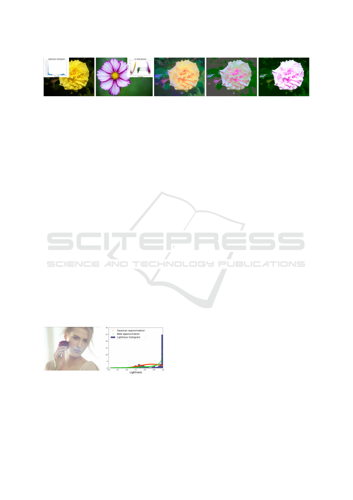
Figure 2: The right-hand plot illustrates the lightness his-
togram of the left-hand image as well as two approxima-
tions, namely Gaussian and Beta. The Gaussian distribution
provides a poor approximation of the asymmetric lightness
distribution. In contrast, the Beta distribution models the
image lightness more accurately by accounting for its right-
skewness.
2 RELATED WORK
This paper presents a novel Beta transformation ap-
plied to color transfer between images. Therefore,
hereafter we discuss existing transformations related
to color transfer. Color transfer methods are gener-
ally classified into statistical methods and geometric
methods (Faridul et al., 2014). In this paper, we focus
on statistical color transformations as they are more
general (i.e. can easily be applied to a variety of image
pairs), content-independent and do not require user
assistance.
Statistical color transformations modify specific
image features, such as color histograms and distribu-
tions. The very first statistical color transfer method
is the non-parametric histogram matching. The lat-
ter transfers the target color palette to the input im-
age by matching the input and target cumulative den-
sity functions. The full histogram transfer often re-
sults in visual artifacts. To resolve this problem,
Pouli et al. (Pouli and Reinhard, 2010; Pouli and
Reinhard, 2011) propose two methods for partial his-
togram matching at different scales.
Furthermore, a number of parametric color trans-
formations have been proposed. They are computed
using the Gaussian distribution. In this sense, Rein-
hard et al. (Reinhard et al., 2001) are the first to as-
sume that each color channel of the input and target
images can be well-described by a univariate Gaus-
sian distribution. They introduce a simple color map-
ping between two Gaussian distributions, which is ap-
plied between each pair of input/target color channels.
This method proves to be effective for natural scenes
but it may introduce false colors in the result.
Reinhard et al.’s transformation is a one-
dimensional transformation which does not take the
correlation between the channels of the color space
into account. To overcome this drawback, Piti
´
e
et al. (Piti
´
e and Kokaram, 2006) propose a three-
dimensional (3D) color transformation. Similarly to
Reinhard et al., Piti
´
e et al. describe the 3D color
Transformation of the Beta Distribution for Color Transfer
113

distributions of the input and target images using
the multivariate Gaussian distribution (MGD). This
helps for their color mapping to be computed as
a closed-form solution to the well-known Monge-
Kantorovich’s optimization problem (Evans, 1997).
Piti
´
e et al.’s color transformation is more robust than
Reinhard et al.’s, as the former minimizes the dis-
placement cost of the color transfer, preventing color
swaps and preserving the intended geometry of the
result.
Despite the efficiency of Piti
´
e et al.’s method, the
global Gaussian assumption may become too strong
to ensure a good color transfer, as shown in fig-
ure 1. To improve the quality of the color transfer, lo-
cal color transfer methods have been introduced (Tai
et al., 2005; Bonneel et al., 2013; Hristova et al.,
2015). Such local methods first partition the input and
target images into several clusters which can be fitted
by an MGD. The clustering is commonly performed
using GMMs (Tai et al., 2005; Hristova et al., 2015).
After the image clustering, either Reinhard et al.’s or
Piti
´
e et al.’s color transformations are carried out be-
tween the corresponding input/target clusters. The re-
sults of the local color transfer methods strongly de-
pend on how the target clusters are mapped to the in-
put ones. For instance, Bonneel et al. (Bonneel et al.,
2013) propose a mapping function based only on the
lightness of the input and target images. Hristova et
al. (Hristova et al., 2015) go further and introduce four
new mapping policies, which are functions of both the
lightness and the chroma of the input and target im-
ages.
Local color transfer methods adopt more pre-
cise distribution models, i.e. GMMs, to fit the input
and target color distributions, which improves signif-
icantly the results of the color transfer, as shown in
figure 1. Evidently, this indicates that the more ac-
curate the adopted distribution model, the better the
results of the color transfer. We believe that we can
further improve the precision of the model by using
the Beta distribution. The Beta distribution can ac-
count for the skewness of the color and light distri-
butions. Moreover, the Beta distribution, which is
bounded, is a more appropriate model for the discrete
color and light distributions of images than the con-
tinuous Gaussian distribution. The following section
presents our novel transformation between two Beta
distributions, which is later applied to color transfer
between images.
3 BETA TRANSFORMATION
The present section consists of two parts: a first
part presenting both the Beta distribution and well-
known statistical transformations of the Beta distribu-
tion, and a second part introducing our Beta transfor-
mation.
3.1 Beta Distribution
First, we present the density function of the Beta
distribution as well as several well-known statistical
transformations which play an important role in the
derivation of our Beta transformation.
3.1.1 Density Function
The density function f (·) of a Beta distributed ran-
dom variable x with shape parameters α, β > 0 (de-
noted x ∼ Beta(α,β)) is given as follows:
f (x) =
1
B(α,β)
x
α−1
(1 −x)
β−1
, (1)
where x ∈ [0,1], and B(α,β) denotes the Beta func-
tion. The Beta distribution is a univariate distribution.
The variable x, distributed according to the Beta law,
can be directly transformed into a Fisher variable us-
ing a simple statistical transformation, as presented
hereafter.
3.1.2 Beta-Fisher Relationship
Let x ∼ Beta(α,β). Then, a variable y, obtained as
y = f
BF
(x,α,β), where function f
BF
(·) is defined as
follows:
f
BF
(x,α,β) =
βx
α(1 −x)
, (2)
is a Fisher variable with shape parameters 2α and
2β (denoted y ∼ F (2α, 2β)). Equation (2) maps the
bounded interval [0, 1] into the semi-bounded interval
[0, ∞) with lim
x→1
y = ∞.
Reversely, a variable z = f
FB
(y,α,β), where
f
FB
(·) is obtained by the following formula:
f
FB
(y,α,β) =
αy
β + αy
, (3)
and y = f
BF
(x,α,β), is a Beta variable, e.g. z ∼
Beta(α,β). Equation (3) maps the semi-founded in-
terval [0, ∞) into the bounded interval [0, 1] with
lim
y→∞
z = 1.
GRAPP 2018 - International Conference on Computer Graphics Theory and Applications
114
u~Beta(α
u
, β
u
)
Beta-to-Fisher:
f
u
:= T
BF
(u)
f
u
~F(2α
u
,2β
u
)
Fisher-to-Beta:
g := T
FB
(f
v
)
g~Beta(α
v
,β
v
)
v~Beta(α
v
, β
v
)
Fisher-to-Standard-Normal:
s
u
:= T
P
(f
u
)
s
u
~N(0,1)
Standard-Normal-to-Fisher:
f
v
:= T
IP
(s)
f
v
~F(2α
v
,2β
v
)
Input image u
Target image v
Output image g
Figure 3: Our Beta transformation consists of four intermediate transformations (steps). The first two steps progressively
transform the input distribution into a standard normal distribution. Then, using the target distribution, the last two trans-
formations reshape the standard normal distribution into a Beta distribution with shape parameters close to the target shape
parameters. For each step of our method, the flowchart shows the transformed distribution and its corresponding approxima-
tion. For illustration’s sake, the input and target distributions are extracted from the lightness channels of two images. The
same sequence of steps can be applied independently to each of the two chroma channels of the input and target images. The
flowchart illustrates one iteration of our method.
3.2 Transformation of the Beta
Distribution
Hereafter, we introduce our one-dimensional (1D)
Beta transformation (it is a transformation between
two univariate Beta distributions). Let u and v be 1D
input and target random variables, following a Beta
distribution, i.e. u ∼ Beta(α
u
, β
u
) and v ∼ Beta(α
v
,
β
v
). We aim to transform variable u so that its dis-
tribution becomes similar to the target distribution
(i.e. the distribution of v).
Transforming one Beta distribution into another
one in a single pass could be challenging. To the
best of our knowledge, no such transformation has yet
been proposed. In this paper, we progressively trans-
form the input Beta distribution by benefiting from
the potential of well-known statistical transformations
and approximations. We propose a transformation of
the Beta distribution, consisting of four intermediate
transformations, as follows:
1. Transformation of the input variable u into a
Fisher variable f
u
∼ F (2α
u
,2β
u
);
2. Transformation of the Fisher variable f
u
into a
standard normal variable s
u
;
3. Transformation of the standard normal variable s
u
into a Fisher variable f
v
∼ F (2α
v
,2β
v
);
4. Transformation of the Fisher variable f
v
into a
Beta variable g ∼ Beta(α
v
,β
v
).
The key idea of our transformation consists in
transforming the input Beta distribution into a stan-
dard normal distribution. The standard normal dis-
tribution can then be easily reshaped using the shape
parameters of the target Beta distribution. However,
the Beta distribution cannot be directly transformed
into a standard normal distribution. To this end, we
first perform an intermediate transformation to com-
pute a Fisher distribution from the input Beta distri-
bution. Then, we use the computed Fisher distribu-
tion to approximate the standard normal distribution.
The output of the proposed transformation is the Beta
variable g which has a distribution similar to the tar-
get Beta distribution. The steps of our transformation
are illustrated in figure 3 and described hereafter.
Transformation of the Beta Distribution for Color Transfer
115

3.2.1 Beta-to-Fisher
During the first step of our transformation, we trans-
form the input Beta variable u into a Fisher variable
f
u
= T
BF
(u) with shape parameters 2α
u
and 2β
u
as
follows:
T
BF
: u → f
BF
(u,α
u
,β
u
), (4)
where function f
BF
(·) is defined in (2). Once we have
obtained the Fisher variable f
u
, we transform it into a
standard normal variable s
u
in the second step of our
transformation.
3.2.2 Fisher-to-Standard-Normal
The transformation of the Fisher variable f
u
, obtained
during the first step of our method, is based on Paul-
son’s equation (Paulson, 1942; Ashby, 1968).
In general, Paulson’s equation transforms a given
Fisher variable f ∼ F (α, β) into a standard normal
variable s ∼ N(0,1) as follows (see appendix A for
a detailed derivation of Paulson’s equation):
s = f
P
(f,µ
x
,µ
y
,σ
x
,σ
y
, p) =
f
1
p
µ
y
−µ
x
q
f
2
p
σ
2
y
+ σ
2
x
, (5)
with σ
2
x
= f
σ
(α, p), σ
2
y
= f
σ
(β, p), µ
x
= f
µ
(σ
x
) and
µ
y
= f
µ
(σ
y
), where p ∈N, and the functions f
σ
(·) and
f
µ
(·) are defined as follows:
f
σ
(γ, p) =
2
γp
2
and f
µ
(σ) = 1 −σ
2
. (6)
We adopt Paulson’s equation (5) to transform the
Fisher variable f
u
∼ F (2α
u
,2β
u
), computed with
transformation (4), into a standard normal variable
s
u
= T
P
(f
u
). The transformation T
P
is defined as fol-
lows:
T
P
: f
u
→ f
P
(f
u
,µ
u
α
,µ
u
β
,σ
u
α
,σ
u
β
, p), (7)
where p ∈ N and (σ
u
α
)
2
= f
σ
(2α
u
, p), (σ
u
β
)
2
=
f
σ
(2β
u
, p), µ
u
α
= f
µ
(σ
u
α
) and µ
u
β
= f
µ
(σ
u
β
). Function
f
P
is defined in (5).
3.2.3 Standard-Normal-to-Fisher
Once we have computed the standard normal variable
s
u
, we inverse Paulson’s equation (5) to transform s
u
into a Fisher variable f
v
. We carry out the inversed
Paulson’s equation using the target shape parameters
α
v
and β
v
instead of the input shape parameters α
u
and β
u
.
Let α and β be any two shape parameters. We
first present the inversed Paulson’s equation for trans-
forming any standard normal variable s into a Fisher
variable f ∼ F (2α,2β):
(s
2
σ
2
y
−µ
2
y
)f
2
p
+ 2µ
x
µ
y
f
1
p
+ s
2
σ
2
x
−µ
2
x
= 0, (8)
where σ
2
x
= f
σ
(2α, p), σ
2
y
= f
σ
(2β, p), µ
x
= f
µ
(σ
x
)
and µ
y
= f
µ
(σ
y
). The solutions of the inversed Paul-
son’s equation are derived in appendix B.
Now, we solve the inversed Paulson’s equation (8)
using the target shape parameters α
v
and β
v
. In (8),
we replace s by s
u
(computed with transformation (7))
and the functions σ
2
x
, σ
2
y
, µ
x
and µ
y
by the following
functions respectively: (σ
v
α
)
2
= f
σ
(2α
v
, p), (σ
v
β
)
2
=
f
σ
(2β
v
, p), µ
v
α
= f
µ
(σ
v
α
) and µ
v
β
= f
µ
(σ
v
β
).
After solving equation (8) using the aforemen-
tioned parameters, we obtain a Fisher variable f
v
∼
F (2α
v
,2β
v
). Each sample f
i
v
of f
v
is computed using
a transformation T
IP
, i.e. f
i
v
= T
IP
(s
i
u
) ∀i ∈{1,...,n}:
T
IP
:
s
i
u
→
f
IP
(s
i
,µ
v
α
,µ
v
β
,σ
v
α
,σ
v
β
,1)
p
,if s
i
u
< 0,
s
i
u
→
f
IP
(s
i
,µ
v
α
,µ
v
β
,σ
v
α
,σ
v
β
,−1)
p
,if s
i
u
≥ 0,
(9)
where p ∈N and function f
IP
(·) is defined in equation
(20) (appendix B).
3.2.4 Fisher-to-Beta
In the final step of our transformation, we transform
the Fisher variable f
v
into a Beta variable g using the
following transformation T
FB
:
T
FB
: f
v
→ f
FB
(f
v
,α
v
,β
v
), (10)
where function f
FB
(·) is defined in (3). The variable
g = T
FB
(f
v
) is approximately distributed according to
a Beta distribution with shape parameters α
v
and β
v
,
i.e. its distribution is similar to the target distribution.
3.2.5 Choice of p
The inverse Paulson’s equation (8) has two solutions
(as shown in appendix B), which can be both negative
and positive, depending on the parameters µ
v
α
, µ
v
β
, σ
v
α
and σ
v
β
. In contrast, the values of the variables, dis-
tributed according to the Fisher law, are non-negative.
To ensure that each component f
i
v
of the Fisher vari-
able f
v
is non-negative (see (9)), we make the param-
eter p equal to 4, following Hawkins et al.’s proposi-
tion (Hawkins and Wixley, 1986). By choosing p = 4,
we also make sure that Paulson’s equation (5) holds
for small values of the shape parameters α
u
and β
u
,
as discussed in (Hawkins and Wixley, 1986).
3.2.6 Iterations
For the sake of robustness, our Beta transformation
can be performed iteratively using a dynamic input
variable. In this case, at the beginning of each itera-
tion (after the first one) the input variable is updated
GRAPP 2018 - International Conference on Computer Graphics Theory and Applications
116

using the resulting variable from the previous itera-
tion, i.e.:
g
(t)
=
(
T
Beta
(u,v),if t = 1;
T
Beta
(g
(t−1)
,v),if t ∈ [2,N],
(11)
where g
(t)
denotes the result after iteration t, T
Beta
de-
notes our Beta transformation (which is a combina-
tion of the four steps, presented earlier in this section)
and N denotes the number of iterations. The benefit of
iterating the proposed transformation and the choice
of an appropriate value for N are discussed in the fol-
lowing section.
3.3 Evaluation of Beta Transformation
To evaluate the performance of our method, we carry
out our Beta transformation on 111 different pairs of
input and target data samples, which we model using
the Beta distribution. The data samples are extracted
from a collection of images containing both indoor
and outdoor images.
We compute the percentage error between the
shape parameters of each resulting (from the trans-
formation) distribution and the target shape parame-
ters. The Box-and-Whisker plots in figure 4 show the
distributions of the percentage errors (for 1 and 5 it-
erations of our transformation). After 1 iteration, the
mean percentage error is less than 0.05 and it con-
verges towards 0 after 5 iterations.
The plots in figure 4 illustrate the benefit of per-
forming our Beta transformation iteratively. After a
single iteration, the mean percentage error is already
significantly small. The more we iterate, the smaller
the mean percentage error. For the application, shown
in this paper (i.e. color transfer), our experiments have
indicated that the change in the distribution of the re-
sult g
(t)
becomes negligible after the fifth iteration,
i.e. for t > 5, as illustrated in figure 5. Therefore, the
results, shown in this paper, are obtained using five
iterations of our Beta transformation, i.e. N = 5.
1 iteration
α
β
0.00 0.05 0.10 0.15
P ercentage error
P ercentage erro r
α
β
0e+00 4e−06 8e−06
5 iterations
Figure 4: Box-and-Whisker plots of the percentage errors
for the two Beta shape parameters α and β (computed after
1 and 5 iterations of our transformation).
4 RESULTS
We apply our Beta transformation in the context of
color transfer between input and target images. We
carry out our 1D Beta transformation independently
on each pair of input/target color channels. To this
end, we use CIE Lab, as the color space provides ef-
ficient channel decorrelation. Each of our results in
this paper is obtained using 5 iterations of our trans-
formation. We perform the Beta transformation glob-
ally (i.e. on the distributions of entire images) as well
as locally (i.e. on the distributions of image clusters).
4.1 Global Color Transfer
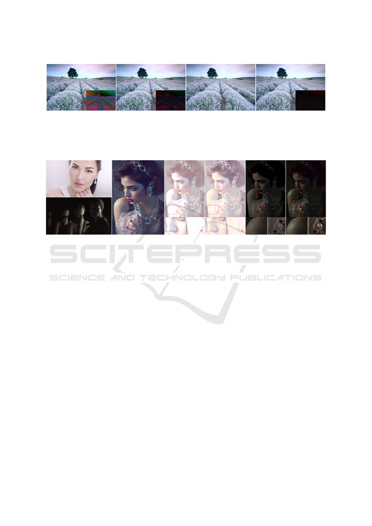
To perform a global color transfer, we first model the
distribution of each input/target channel by a Beta dis-
tribution and then, we carry out our Beta transforma-
tion between the channel distributions. In figure 6,
our global Beta-based color transfer is compared to
the Gaussian-based 3D linear color transformation by
Piti
´
e et al. (Piti
´
e and Kokaram, 2006) (also carried
out in CIE Lab). Target image (a) is a highly bright
image, characterized by a low contrast (i.e. there is an
absence of strongly defined highlights). Similarly, our
first result in figure 6 does not contain highly contrast-
ing regions, i.e. the illumination of our result appears
uniform (much like the illumination of target image
(a)). Moreover, our first result has a lower contrast
than the input image but it looks sharper than its cor-
responding result by Piti
´
e et al. We observe that our
result (a) preserves more details from the input im-
age (note the sharpness of the girl’s face and hair in
our first result). In contrast, Piti
´
e et al.’s first result
contains regions of over-saturated pixels, appearing
on the girl’s face, shoulder and flower (snippets (1)
and (2)), causing a loss of details. Such highlights are
uncharacteristic for target image (a) and their pres-
ence increases the contrast of Piti
´
e et al.’s result.
Furthermore, target image (b) in figure 6 is char-
acterized by a presence of strong highlights and deep
shadows. Likewise, highly contrasting regions appear
in our result (b), whereas the absence of strong high-
lights in Piti
´
e et al.’s result (b) influences the contrast
decrease and makes the image appear flat.
4.2 Local Color Transfer
Instead of modeling the entire distributions of color
and light by Beta distributions, we can build an
even more accurate model using Beta mixture models
(BMMs) (Ma and Leijon, 2009). We use BMMs to
cluster the input and target images according to one
of two components, i.e. lightness or hue. We adopt
Transformation of the Beta Distribution for Color Transfer
117
1 iteration
2 iterations
5 iterations
10 iterations
Figure 5: Results of our Beta transformation (applied iteratively in the context of color transfer between images) for different
number of iterations. Bottom-right corner: images of the observed difference between each result and the result, obtained after
the fifth iteration. As observed, the more we iterate, the smaller the difference. The difference between the result, obtained
after the fifth iteration, and the result, obtained after the tenth iteration, is negligible and therefore, we can assume that our
method converges after the fifth iteration (this conclusion has been drawn using various results of color transfer). The input
and target images for the color transfer are presented in figure 3.
Input imageTarget image
[Pitie et al., 2007] [Pitie et al., 2007]
Our result Our result
(a)
(b)
(a) (a)
(b) (b)
(1) (2) (1) (2)
(1) (2) (1) (2)
(2) (2)
(1) (1)
(1) (1)
(2)(2)
Figure 6: Global color transfer. Our results portray the contrast of the target image better than the Piti
´
e et al.’s results and they
appear sharper than Piti
´
e et al.’s results. Snippets (1) and (2) illustrate differences between our results and Piti
´
e et al.’s results
(best viewed on screen).
the classification method, proposed in (Hristova et al.,
2015), to determine the best clustering component for
each image. Additionally, we let clusters overlap and
we use the BMMs soft segmentation to compute the
overlapping pixels. Then, we apply the mapping poli-
cies, proposed in (Hristova et al., 2015), to map the
target to the input clusters and we carry out our Beta
transformation between each pair of corresponding
clusters (see (Hristova et al., 2015)). The overlapping
pixels are influenced by more than one Beta transfor-
mation. To determine the final value of an overlap-
ping pixel, we compute the average of all transforma-
tions, containing the pixel, using exponential decay
weights like in (Hristova et al., 2015).
Figure 7 illustrates the benefit of applying a local
color transfer between images. In figure 7, our global
Beta transformation fails to transfer properly the tar-
get color palette to the input image. This is due to the
fact that the color distributions of the input and target
images in figure 7 cannot be modelled well enough
by a single Beta distribution. To improve the result of
the global transfer, we apply our Beta transformation
locally, using 2 clusters. That way, BMMs, as more
precise distribution models for the input/target distri-
butions, help to transfer the target colors more accu-
rately. We compare our local method with Bonneel et
al.’s (Bonneel et al., 2013) and Hristova et al.’s (Hris-
tova et al., 2015) local methods, both of which per-
form clustering and carry out Gaussian-based trans-
formations. As shown in figure 7, Bonneel et al.’s
method fails to match the target floral color (making
the flower in the result appear less white and slightly
saturated), whereas Hristova et al.’s method causes
overexposure of the foreground pixels in the result.
In contrast, our local result portrays the natural cream
white color of the target rose without overexposing it.
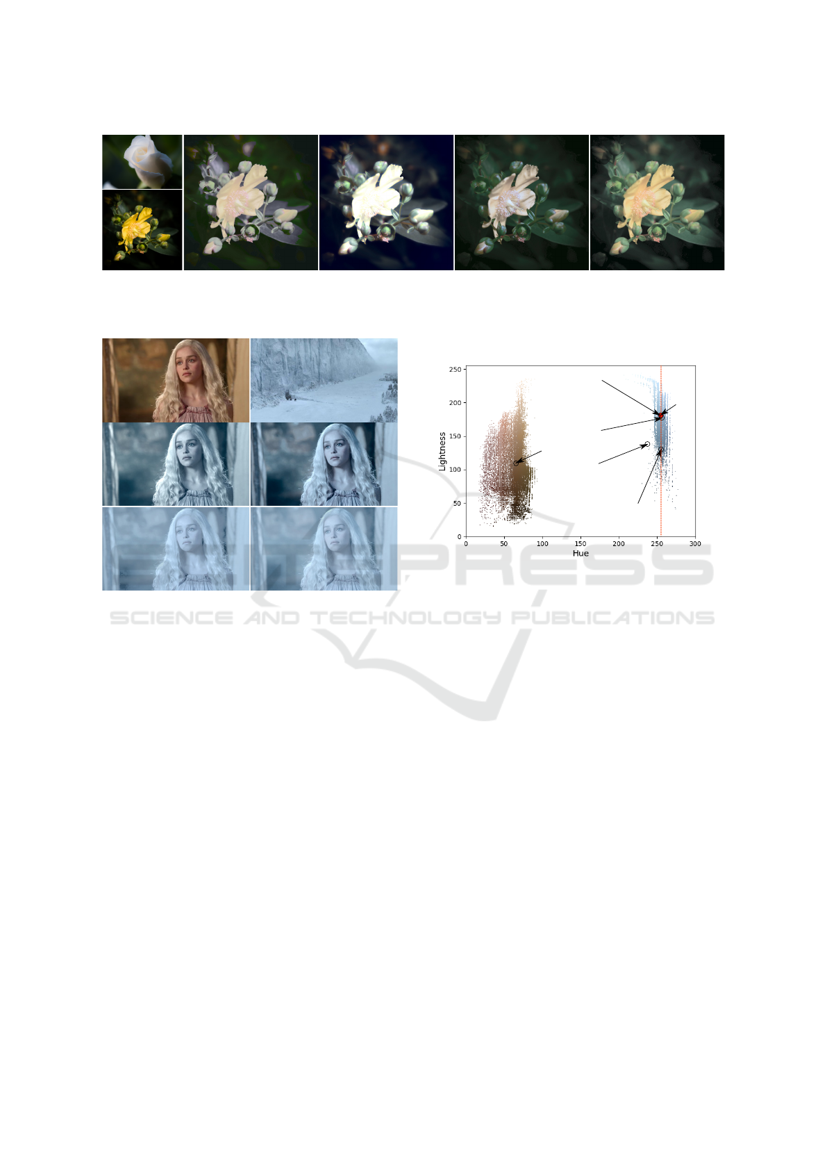
Furthermore, our local Beta transformation can
also influence the contrast of the result. For instance,
figure 8 shows that when we apply our Beta trans-
formation globally, we accurately transfer the target
color palette. However, that way we also decrease
the contrast of the result, making it appear unnaturally
under-saturated. Due to the specific contents of the in-
put/target images in figure 8, users may expect a more
saturated result with a higher contrast. To preserve the
input contrast, we perform our Beta transformation
locally using two lightness clusters, i.e. highlights and
shadows. That way, we can transfer the target colors
without compromising the input contrast.
As the input and target images in figure 8 consist
of a single dominant color, the average hue provides
a decent statistic for measuring the similarity of each
GRAPP 2018 - International Conference on Computer Graphics Theory and Applications
118
Our result, 2 clusters
[Bonneel et al., 2013]
[Hristova et al., 2015]
Input image
Target image
Our result, 1 cluster
Figure 7: Local color transfer. The local Beta transformation is more efficient than the global Beta transformation in cases
when the input/target color and light distributions cannot be well-modelled by a single Beta distribution. We use 2 clusters to
obtain a naturally-looking result, matching accurately the target color palette and contrast.
Input image
Target image
[Bonneel et al., 2013]
[Hristova et al., 2015]
Our result, 2 clusters
Our result, 1 cluster
Figure 8: Our local color transfer may significantly influ-
ence the contrast of the resulting image. Our global method
accurately transfers the target color palette, but it also de-
creases the contrast, resulting in an unnaturally flat image.
On the other hand, our local Beta transformation preserves
the input contrast.
result to the target color palette. Figure 9 presents a
plot of the lightness-hue distributions of the input and
target images appearing in figure 8. In the plot of fig-
ure 9, the mean lightness and the mean hue of each
result in figure 8 are displayed in circles. We observe
that our local result, obtained using two clusters, has
the same mean hue as the target image. In contrast,
Hristova et al.’s result has an out-of-gamut mean hue.
Indeed, a closer visual comparison between our local
result and Hristova et al.’s result (figure 8) indicates
that our local method transfers the target color palette
more accurately (note the slightly different (from the
target image) shade of blue in Hristova et al.’s result).
The hue statistic supports this observation: our local
result matches the target colors better than Hristova
et al.’s result. Furthermore, the difference between
our local result and the target image in terms of mean
lightness is expected and can be explained by the in-
tentional preservation of the input contrast. Finally,
Our result, 1 cluster
Our result, 2 clusters
[Hristova et al., 2015]
[Bonneel et al., 2013]
Target
Input
Figure 9: Lightness-hue distribution plot of the input and
target images from figure 8. The left cluster corresponds to
the color distribution of the input image, whereas, the right
cluster corresponds to the color distribution of the target im-
age. The red circle illustrates the mean target lightness and
hue, whereas the dashed red line visualizes the mean target
hue.
more results, obtained with our local Beta transfor-
mation, are presented in figure 10.
5 CONCLUSION AND FUTURE
WORK
In this paper, we have presented a transformation be-
tween two Beta distributions. Our main idea involved
modelling color and light image distributions using
the Beta distribution (or BMMs) as an alternative to
the Gaussian distribution (or GMMs). We have ap-
plied our Beta transformation in the context of color
transfer between images, though the transformation
can be applied to any bounded data, following the
Beta distribution law. Our results have shown the ro-
bustness of our method for transferring given target
color palette and contrast.
The proposed 1D Beta transformation has been
Transformation of the Beta Distribution for Color Transfer
119

Target image (a) Target image (b)
Result (a) Result (b)
Input image
Figure 10: More results, obtained with our Beta transformation. We apply our Beta transformation locally using two clusters
(either lightness or hue clusters). The mapping between the input/target clusters is carried out using the mapping policies,
proposed in (Hristova et al., 2015).
applied on each input channel separately without ac-
counting for the channels inter-dependency. The lat-
ter highlights the main limitation of our method. To
improve the results of our method, we can extend the
dimensionality of our Beta transformation by consid-
ering the Dirichlet distribution. The Dirichlet distri-
bution (Kotz et al., 2004) is the multivariate general-
ization (for more than two shape parameters) of the
Beta distribution. The Dirichlet distribution with four
shape parameters could be used to model any three-
dimensional data, such as the joint 3D distribution of
color and light in images. Given the promising color
transfer results, obtained using our Beta transforma-
tion, we believe that the Dirichlet distribution would
also prove beneficial to image editing and that is why,
we consider it as a future avenue for improvement.
REFERENCES
Ashby, T. (1968). A modification to paulson’s approxima-
tion to the variance ratio distribution. The Computer
Journal, 11(2):209–210.
Bonneel, N., Sunkavalli, K., Paris, S., and Pfister, H. (2013).
Example-based video color grading. ACM Transac-
tions on Graphics (Proceedings of SIGGRAPH 2013),
32(4):2.
Evans, L. C. (1997). Partial differential equations and
monge-kantorovich mass transfer. Current develop-
ments in mathematics, 1999:65–126.
Faridul, H. S., Pouli, T., Chamaret, C., Stauder, J., Tr
´
emeau,
A., Reinhard, E., et al. (2014). A survey of color map-
ping and its applications. In Eurographics 2014-State
of the Art Reports, pages 43–67. The Eurographics
Association.
Fieller, E. (1932). The distribution of the index in a normal
bivariate population. Biometrika, pages 428–440.
Hawkins, D. M. and Wixley, R. (1986). A note on the trans-
formation of chi-squared variables to normality. The
American Statistician, 40(4):296–298.
Hristova, H., Le Meur, O., Cozot, R., and Bouatouch, K.
(2015). Style-aware robust color transfer. EXPRES-
SIVE International Symposium on Computational
Aesthetics in Graphics, Visualization, and Imaging.
Hwang, Y., Lee, J.-Y., Kweon, I. S., and Kim, S. J.
(2014). Color transfer using probabilistic moving least
squares. In Computer Vision and Pattern Recogni-
tion (CVPR), 2014 IEEE Conference on, pages 3342–
3349. IEEE.
Kotz, S., Balakrishnan, N., and Johnson, N. L. (2004). Con-
tinuous multivariate distributions, models and appli-
cations. John Wiley & Sons.
Ma, Z. and Leijon, A. (2009). Beta mixture models and the
application to image classification. In Image Process-
ing (ICIP), 2009 16th IEEE International Conference
on, pages 2045–2048. IEEE.
Oliveira, M., Sappa, A. D., and Santos, V. (2011). Unsu-
pervised local color correction for coarsely registered
images. In Computer Vision and Pattern Recognition
(CVPR), 2011 IEEE Conference on, pages 201–208.
IEEE.
Olkin, I. and Pukelsheim, F. (1982). The distance between
two random vectors with given dispersion matrices.
Linear Algebra and its Applications, 48:257–263.
Paulson, E. (1942). An approximate normalization of the
analysis of variance distribution. The Annals of Math-
ematical Statistics, 13(2):233–235.
Piti
´
e, F. and Kokaram, A. (2006). The linear monge-
kantorovitch linear colour mapping for example-based
colour transfer. In CVMP’06. IET.
Pouli, T. and Reinhard, E. (2010). Progressive histogram
reshaping for creative color transfer and tone repro-
duction. In Proceedings of the 8th International Sym-
posium on Non-Photorealistic Animation and Render-
ing, pages 81–90. ACM.
Pouli, T. and Reinhard, E. (2011). Progressive color transfer
GRAPP 2018 - International Conference on Computer Graphics Theory and Applications
120

for images of arbitrary dynamic range. Computers &
Graphics, 35(1):67–80.
Reinhard, E., Adhikhmin, M., Gooch, B., and Shirley, P.
(2001). Color transfer between images. Computer
Graphics and Applications, IEEE, 21(5):34–41.
Shih, Y., Paris, S., Durand, F., and Freeman, W. T. (2013).
Data-driven hallucination of different times of day
from a single outdoor photo. ACM Transactions on
Graphics (TOG), 32(6):200.
Tai, Y.-W., Jia, J., and Tang, C.-K. (2005). Local color
transfer via probabilistic segmentation by expectation-
maximization. In Computer Vision and Pattern Recog-
nition, 2005. CVPR 2005. IEEE Computer Society
Conference on, volume 1, pages 747–754. IEEE.
APPENDICES
A: Paulson’s Equation
Hereafter, we derive Paulson’s equation (5). First,
we present a well-known transformation of the Fisher
distribution, which plays a key role for the derivation
of Paulson’s equation.
Fisher-Chi-square Relationship. A Fisher variable
can be expressed as a ratio of two Chi-square vari-
ables. Let x and y be two Chi-square random vari-
ables with α and β degrees of freedom respectively
(x ∼ χ
2
α
, y ∼ χ
2
β
). Then:
x/α
y/β
∼ F (α,β). (12)
Normal-Chi-square Relationship. Let z ∼ N(µ,σ
2
)
be a normal variable and w ∼χ
2
γ
be a Chi-square vari-
able with γ degrees of freedom. Then, z can be ex-
pressed as follows (Hawkins and Wixley, 1986):
z =
w
γ
1
p
, (13)
where p ∈ N and µ and σ are functions of γ and p:
σ
2
= f
σ
(γ, p) and µ = f
µ
(σ). (14)
Functions f
σ
(·) and f
µ
(·) are defined in (6).
Derivation of Paulson’s Equation. We derive Paul-
son’s equation using Fieller’s approximation (Fieller,
1932). Fieller’s approximation transforms the ratio
of two normally distributed variables into a standard
normal variable. Let x ∼N(µ
x
,σ
2
x
) and y ∼ N(µ
y
,σ
2
y
)
be two normally distributed random variables. Then,
Fieller approximation (Fieller, 1932) admits the fol-
lowing form:
s = f
FL
(x,y,µ
x
,µ
y
,σ
x
,σ
y
) =
x
y
µ
y
−µ
x
r
x
y
2
σ
2
y
+ σ
2
x
(15)
Variable s, where s = f
FL
(x,y,µ
x
,µ
y
,σ
x
,σ
y
), is a
standard normal variable.
Paulson’s equation can be derived from (15) by
computing the normal variables x and y using the Chi-
square distribution. In this sense, we express the nor-
mal variables x and y in (15) using equation (13) as
follows:
x = (w
x
/α)
1
p
and y = (w
y
/β)
1
p
, (16)
where w
x
∼ χ
2
α
and w
y
∼ χ
2
β
, and p ∈ N. Then, we
compute a new variable f as follows:
f =
x
p
y
p
=
w
x
/α
w
y
/β
. (17)
From (12), it becomes clear that f is a Fisher variable
with shape parameters α and β, i.e. f ∼F (α,β). Once
we have replaced the ratio x/y in Fieller’s approxima-
tion (15) by its equivalence from equation (17), we
obtain Paulson’s equation (5). Paulson’s equation (5)
transforms a Fisher variable into a standard normal
variable.
B: Inversed Paulson’s Equation
For each pair of shape parameters (α, β) and each
standard normal variable s, the inversed Paulson’s
equation (8) can be solved as a quadratic equation for
t = f
1
p
. Let t = (t
1
,...,t
n
) and s = (s
1
,...,s
n
), where
t
i
and s
i
are the samples of t and s respectively. Then,
the two solutions t
1
and t
2
of (8) are computed ∀i ∈
{1,...,n} using a function f
IP
(s
i
,µ
x
,µ
y
,σ
x
,σ
y
,C)
(Ashby (Ashby, 1968) presents the solutions for p =
3):
f
1
p
1
= t
1
= f
IP
(s
i
,µ
x
,µ
y
,σ
x
,σ
y
,1), (18)
f
1
p
2
= t
2
= f
IP
(s
i
,µ
x
,µ
y
,σ
x
,σ
y
,−1), (19)
where the function f
IP
(·) is defined as follows:
f
IP
(s
i
,µ
x
,µ
y
,σ
x
,σ
y
,C) =
−µ
x
µ
y
+C
√
D
s
2
i
σ
2
y
−µ
2
y
(20)
for determinant D: D = s
2
i
(σ
2
x
+σ
2
y
+σ
2
x
σ
2
y
(σ
2
x
+σ
2
y
−
s
2
i
−4)), and coefficient C = ±1.
Transformation of the Beta Distribution for Color Transfer
121
