Infrared Image Enhancement in Maritime Environment with

Convolutional Neural Networks

Purbaditya Bhattacharya

, J

org Riechen

and Udo Z

olzer

Department of Signal Processing and Communications, Helmut Schmidt University, Hamburg, Germany

WTD 71 Military Service Center for Ships, Naval Weapons, Maritime Technology and Research, Eckernf

orde, Germany

Keywords:

Image Processing, Convolutional Neural Network, Denoising, Super-resolution.

Abstract:

Image enhancement approach with Convolutional Neural Network (CNN) for infrared (IR) images from mar-

itime environment, is proposed in this paper. The approach includes different CNNs to improve the resolution

and to reduce noise artefacts in maritime IR images. The denoising CNN employs a residual architecture

which is trained to reduce graininess and ﬁxed pattern noise. The super-resolution CNN employs a similar ar-

chitecture to learn the mapping from a low-resolution to multi-scale high-resolution images. The performance

of the CNNs is evaluated on the IR test dataset with standard evaluation methods and the evaluation results

show an overall improvement in the quality of the IR images.

1 INTRODUCTION

Optical cameras contain sensors that are able to de-

tect light of wavelength in the range of 450 - 750 nm

and hence limited by the availability of light. Infrared

(IR) cameras and thermographic cameras in particular

have sensors that detect thermal radiation and are in-

dependent from the amount of ambient visible light.

The thermal radiation of the object determines how

salient or detailed it will be in an infrared image and

can provide useful information, otherwise not avail-

able in a normal image. IR imagery has become con-

siderably popular over the last years because of its us-

age in multiple ﬁelds of application including medical

imaging, material testing, military surveillance. Due

to its effectiveness, IR imaging is used extensively

in maritime environment for maritime safety and se-

curity application, activity detection, object tracking,

and environment monitoring.

IR images suffer from low signal-to-noise ratio

(SNR) because of the non-uniformity of the detec-

tor array responses and their underlying processing

circuits. The ambient temperature plays a very im-

portant role since the IR camera has to be calibrated

accordingly (Zhang et al., 2010). In this context,

outdoor maritime environment poses a bigger chal-

lenge compared to an indoor environment due to the

temperature ﬂuctuations, atmospheric loss, wind, and

rain. In spite of regular camera calibrations and er-

ror correcting techniques (Zhang et al., 2010), the

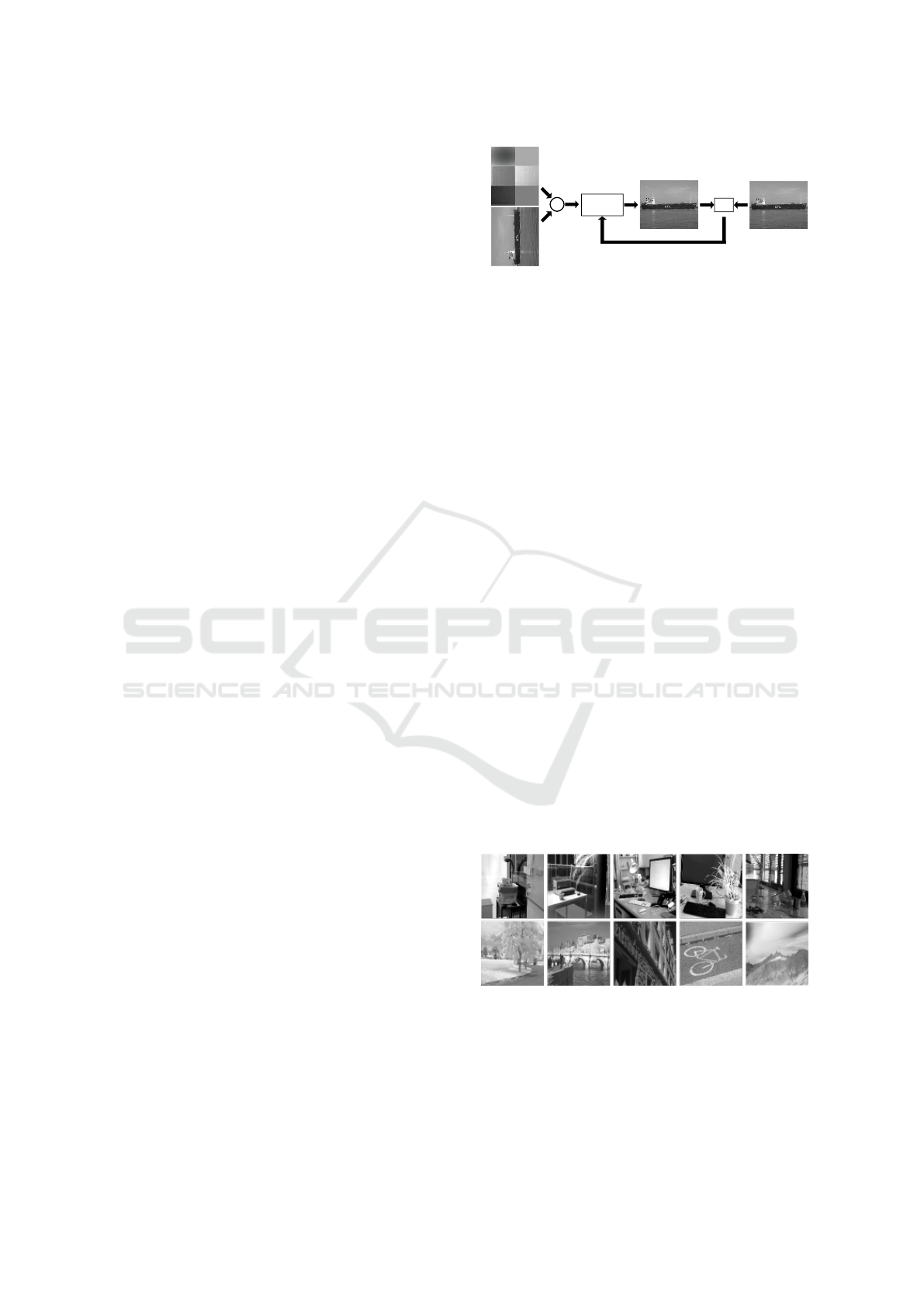
(a) Original (b) Enhanced

Figure 1: An example of enhancement in IR images.

image suffers from spot noise, ﬁxed pattern noise,

graininess, blur and other artefacts. Traditional digital

image processing techniques of image enhancement

have been extensively used over the years. The classi-

cal approaches include the usage of adaptive median

ﬁlters, gradient based approach like the total varia-

tion denoising (Micchelli et al., 2011), (Goldstein and

Osher, 2009), wavelet based approach (Zhou et al.,

2009), non-local self similarity (NSS) based methods

(Dabov et al., 2007), (J.Xu et al., 2015), and meth-

ods on sparse representation based dictionary learning

Bhattacharya, P., Riechen, J. and Zölzer, U.

Infrared Image Enhancement in Maritime Environment with Convolutional Neural Networks.

DOI: 10.5220/0006618700370046

In Proceedings of the 13th International Joint Conference on Computer Vision, Imaging and Computer Graphics Theory and Applications (VISIGRAPP 2018) - Volume 4: VISAPP, pages

37-46

ISBN: 978-989-758-290-5

(Elad and Aharon, 2006). In recent years deep learn-

ing has become a very popular topic due to its success

in solving many computer vision problems. Convolu-

tional neural network (CNN) is the most popular deep

learning tool and has been employed already in many

image enhancement problems e.g., denoising, super-

resolution, and compression artefact removal. This

paper applies a deep learning approach with CNNs to

solve the enhancement problem in maritime IR im-

ages. An example is shown in Figure 1.

2 RELATED WORK

The present work is inﬂuenced by the recent suc-

cess of CNNs in image super-resolution and denois-

ing problems. An artiﬁcial neural network is used

for image denoising in (Jain and Seung, 2009). It is

shown in (Burger et al., 2012) that multi layer per-

ceptrons (MLP) can outperform state-of-the-art stan-

dard denoising techniques. In the area of resolution

improvement, the ”Super-Resolution Convolutional

Neural Network” (SRCNN) (Dong et al., 2015) has

trained a CNN architecture to learn the mapping be-

tween a low and high resolution image. The end to

end learning has yielded very good results but the cor-

responding training convergence is slow. In (He et al.,

2016) it is already established that residual connec-

tions or skip connections in a network increase the

learning speed and improve the overall performance.

Residual networks are particularly useful if the train-

ing data and the ground truth data have high corre-

lation. In this context, CNNs with residual learn-

ing has yielded better results from the perspective of

speed and accuracy. In (Kim et al., 2016) it is estab-

lished that the super-resolution with a deep residual

architecture subsequently improved the performance.

Recently residual learning for image denoising with

CNNs have been used successfully in (Pan et al.,

2016) and (Zhang et al., 2017). Due to the improved

performance of residual networks the present work

has employed residual architectures for the enhance-

ment application.

3 PROPOSED APPROACH

A CNN is a layered architecture primarily compris-

ing of linear multi dimensional convolution kernels

and non-linear activation functions usually appear-

ing alternately in a basic architecture. Apart from

the two layers mentioned, other important layers in-

clude pooling, batch normalization, and fully con-

nected layers and the usage of these layers depends

Label

Output

Update

Input

Blur

Noise Patch

CNN

Loss

Figure 2: An overview of the denoising method.

on the computer vision application. The layers are ar-

ranged in different combinations to create ﬂexible net-

work architectures that are trained iteratively with an

objective function to solve different computer vision

problems. In order to perform a supervised training of

a CNN, it is necessary to create a dataset of image and

ground truth pairs. The purpose of the training is to

learn and generalize the relationship between the im-

ages and the corresponding ground truth images in the

dataset. The dataset is usually divided into training,

validation and test data. The ﬁnal goal of a trained

CNN is to perform the desired action on an unseen

test data. The following sections provide the details

of the denoising and super-resolution CNNs.

3.1 Denoising Method

The denoising method overview is shown in Figure 2.

In the ﬁrst step the dataset is prepared for the denois-

ing task. The primary goal of this work is to suc-

cessfully denoise the IR images from the WTD 71

dataset. For training the CNN the RGB-NIR scene

database (Brown and S

usstrunk, 2011) from the EPFL

Lausanne is used. The database contains a collection

of near infrared (NIR) and color images of indoor and

outdoor scenes from which the NIR images are used

for training. In the second step the CNN is described,

setup and trained.

3.1.1 Data Preparation

Figure 3: Sample clean images from the RGB-NIR training

dataset.

From the RGB-NIR database 400 images and 60 im-

ages are selected for training and validation respec-

tively. To create the training and validation dataset

the clean NIR images are initially resampled and de-

graded with noise to create the input dataset for the

VISAPP 2018 - International Conference on Computer Vision Theory and Applications

Loss

ReLU

Conv

Input

Output

Label

Conv

2121

Figure 4: The architecture of denoising CNN.

CNN, and the clean NIR images are used as the

ground truth or reference dataset. Figure 3 shows

some example images from the database. A majority

of the test IR images from WTD 71 have noisy arte-

facts of varying intensities and properties. A consid-

erable number of noise patches are extracted from the

IR images from areas of uniform background intensi-

ties. Additionally, noisy frames from videos with uni-

form background, containing 35 mm ﬁlm grain, are

extracted and added to the collection of noise patches.

During the creation of the CNN dataset, the noise

patches are randomly augmented and are added to the

clean images after mean subtraction and resizing to

produce the noisy images. The image and ground

truth image pairs of both training and validation data

are divided into patches of 21×21 pixels to create the

ﬁnal dataset. During the training process the image

patches are randomly ﬂipped.

3.1.2 Network Architecture

The example architecture for denoising is shown in

Figure 4. As illustrated in the ﬁgure, the network

is composed of alternate convolutional (Conv) layers

and rectiﬁed linear units (ReLU), with the exception

of the ﬁrst two layers which are convolutional. The

network is only composed of Conv layers and ReLU

layers. There are 7 Conv layers and 5 ReLU layers

in the network and 13 layers altogether including the

Loss layer. The Conv layer performs linear convolu-

tion on each incoming feature map tensor or a tensor

of input image patch with the deﬁned kernels to pro-

duce the output feature maps. As shown in Figure 4

the depth of the convolution kernel should match the

depth of the input feature map and the depth of the

output feature map tensor is equal to the number of

kernels in the Conv layer. Hence the number of ker-

nels used in the ﬁnal Conv layer should be 1 in or-

der to obtain a target output image with a depth or

channel of 1. The convolution operation in each Conv

layer also retains the height and the width of the in-

put feature map to that layer by correct padding. The

depth of the convolution kernel is equal to the depth of

the input feature map tensor. Thus a convolution of a

21×21×1 image patch with 49 kernels of size 7×7×1

produces a feature map tensor of size 21×21×49 in

the ﬁrst layer. The ﬁrst two Conv layers use 7×7×1

and 3×3×49 kernels respectively and the last Conv

layer uses 3×3×64 kernel. The kernels in the ﬁrst

Conv layer are initialized with sparse matrices where

most of the elements are zero valued and the remain-

ing elements have a value of 1. The remaining Conv

layers use 5×5×64 kernels with ReLU layers in be-

tween. The ReLU layer truncates the negative values

in a feature map as given by,

y = max(0, x), (1)

where x denotes the input to the ReLU function, y

denotes the output of the ReLU function, and max

denotes the maximum operator. Before the Loss

layer the input is added to the output so that the net-

work learns to estimate the noise residue. Table 1

shows the information about the network architec-

ture, where Id. denotes the layer index, and w and

b denote weight and bias respectively. The table

also provides the size of each kernel in the form of

height×width×depth×number of kernels. The leak-

age factor (Lk) of the ReLU layer weights the neg-

ative values from the input feature maps instead of

truncating them.

3.1.3 Objective

The objective of the training process is to minimize

a combination of losses deﬁned by the correspond-

ing loss functions. The CNN is trained iteratively to

minimize a weighted combination of loss functions in

order to ﬁnd an optimal solution of the free or train-

able parameters. The combination consists of the L

and L

regression loss functions which operate pixel

wise. The individual loss functions are given in the

below equations,

(y, ˆy) =

||y − ˆy||

, (2)

Infrared Image Enhancement in Maritime Environment with Convolutional Neural Networks

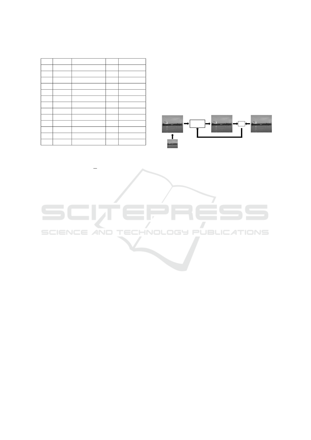
Table 1: The denoising CNN architecture.

Id. Name Kernel Size Lk lr (w, b)

1 Conv 7×7×1×49 - 1e-4, 1e-4

2 Conv 3×3×49×64 - 1e-2, 1e-4

3 ReLU - 0.2 -

4 Conv 5×5×64×64 - 1e-2, 1e-4

5 ReLU - 0.2 -

6 Conv 5×5×64×64 - 1e-2, 1e-4

7 ReLU - 0.2 -

8 Conv 5×5×64×64 - 1e-2, 1e-4

9 ReLU - 0.2 -

10 Conv 5×5×64×64 - 1e-2, 1e-4

11 ReLU - 0.2 -

12 Conv 3×3×64×1 - 1e-2, 1e-4

13 Loss - - -

and

(y, ˆy) =

||y − ˆy||

, (3)

where ˆy denotes the estimated CNN output, y denotes

the ground truth data, and V denotes the volume of

the CNN output or the ground truth data tensor. The

advantage of the L

loss is that it has edge preserving

qualities since the L

norm solves for the median. The

optimization problem is given by,

ˆy = f

(x), (4)

∗

= arg min E

y, ˆy

[

∑

i=1

(y, ˆy))], (5)

where, θ

∗

denotes the optimal solution of the free

or trainable parameters denoted by θ, f

denotes the

CNN model, x denotes the input image, L

(·) denotes

a loss function, α

is the weighting factor for com-

bining the K loss functions, and E

y, ˆy

[·] denotes the

expected value of the combination of loss functions.

From the loss layer the gradients starts backpropa-

gating through each layer following the chain rule of

derivatives. The kernel weights are then updated with

the calculated gradients for the corresponding layers

and the amount of update is controlled by a user spec-

iﬁed learning rate parameter. In order to update the

weights, the adaptive momentum (Adam) optimiza-

tion (Kingma and Ba, 2014) is used, due to its fast

convergence. The weights of the Conv layers are ini-

tialized with Xavier initialization (Glorot and Bengio,

2010) and the weight decay regularization parameter

of 0.001 is used to counter overﬁtting problems. It is

noteworthy that a CNN is usually not trained with one

image per iteration but with a batch of images as de-

termined by a user speciﬁed batch size. Images inside

a batch are randomly selected from the entire dataset

which leads to the stochastic nature of the training

process. In this case a batch size of 64 is used during

the training. During the training process, the learn-

ing rates as shown in Table 1 are adapted by reducing

them by a factor of 2 at every 10th epoch. The net-

work is trained for 90 epochs.

3.2 Super-resolution Method

Label

Output

Update

Bicubic

CNN

Loss

Input

Figure 5: An overview of the super-resolution method.

In this section the CNN model for super-resolution is

described. For super-resolution the RGB-NIR dataset

is used as well. The method overview is shown in

Figure 5. The model for the super-resolution CNN has

differences from the denoising CNN in terms of the

network architecture and data preparation.

3.2.1 Data Preparation

The dataset is prepared with 360 training images and

60 validation images. The training is performed with

both the NIR images as well as with the Y channel of

the color images converted to YCbCr, with the results

from the latter being discussed in this work because

of more stable performance. To create the training

and validation dataset the clean images are initially

resampled with bicubic interpolation to create the in-

put dataset for the CNN and the clean images are used

as the ground truth data. The CNN is trained with re-

sampling factors of 2, 3, and 4 separately. The image

and ground truth pairs of both training and validation

data are divided into patches of 224×224 pixels to

create the ﬁnal dataset. During the training process

the image patches are randomly ﬂipped as a form of

batch augmentation.

3.2.2 Network Architecture

The CNN architecture example for super-resolution

is shown in Figure 6. The network is primarily com-

posed of alternate Conv and ReLU layers and a con-

catenation (Concat) layer. The network has 13 Conv

layers, 12 ReLU layers, 1 Concat layer, and has 27

layers in total including the Loss layer. Each Conv

layer uses 3×3×64 kernel except the ﬁrst layer which

uses a 5×5×1 kernel and the layer after the Concat

VISAPP 2018 - International Conference on Computer Vision Theory and Applications

Loss

ReLUReLU

Conv

Concat

Conv

Input

Output

Label

224

64 64 64 64 64

224

Figure 6: The architecture of super-resolution CNN.

layer which uses 5×5×320 kernel. All the layers em-

ploy 64 The learning rate (lr) of the Conv layers is the

same. Before the last 2 Conv layers there is a Con-

cat layer that collects feature maps from selected lay-

ers along the 3rd dimension of the feature tensor, as

shown in Figure 6. In this particular case the feature

maps from layers 6, 10, 14, 18, and 22, of a depth

of 64 each, are concatenated along the 3rd dimen-

sion of the feature tensor resulting in a feature tensor

with a depth of 320. The Concat layer ensures that

the inference be made from feature maps from layers

of multiple depths and hence multiple resolution with

respect to the information content. The original im-

age is added to the output by a skip connection and

the network learns to estimate the residual high fre-

quency details of the image. Table 2 shows the infor-

mation about the network architecture. As mentioned

previously the depth of the kernel in each Conv layer

equals the depth of the corresponding input feature

map. Hence, the kernel depth in the Conv layer fol-

lowing the Concat layer is 320 as given in Table 2.

For super-resolution factors of 3 and 4, the same net-

work architecture with different kernel depths (32), is

used.

3.2.3 Objective

The super-resolution CNN is trained with a similar

combination of loss functions as in the case of de-

noising. The goal of the training is to minimize the

expected combined loss as given in Equation (5). The

weights of the Conv layers are initialized with the im-

proved Xavier initialization. The weight decay regu-

larization parameter of 0.0005 is used and a batch size

of 8 is used during training. The Adam optimizer is

used to update the weights and biases in the Conv lay-

ers. During the training, the learning rate is adapted

by reducing it by a factor of 2 after every 20th epoch.

Training of the network with different resampling fac-

tors are performed separately for 230 epochs.

Table 2: The super-resolution CNN architecture.

Id. Name Kernel Size Lk lr (w, b)

1 Conv 5×5×1×64 - 1e-2, 1e-5

2 ReLU - 0 -

3 Conv 3×3×64×64 - 1e-2, 1e-5

4 ReLU - 0 -

5 Conv 3×3×64×64 - 1e-2, 1e-5

6 ReLU - 0 -

7 Conv 3×3×64×64 - 1e-2, 1e-5

8 ReLU - 0 -

9 Conv 3×3×64×64 - 1e-2, 1e-5

10 ReLU - 0 -

11 Conv 3×3×64×64 - 1e-2, 1e-5

12 ReLU - 0 -

13 Conv 3×3×64×64 - 1e-2, 1e-5

14 ReLU - 0 -

15 Conv 3×3×64×64 - 1e-2, 1e-5

16 ReLU - 0 -

17 Conv 3×3×64×64 - 1e-2, 1e-5

18 ReLU - 0 -

19 Conv 3×3×64×64 - 1e-2, 1e-5

20 ReLU - 0 -

21 Conv 3×3×64×64 - 1e-2, 1e-5

22 ReLU - 0 -

23 Concat - - -

24 Conv 3×3×320×64 - 1e-2, 1e-5

25 ReLU - 0 -

26 Conv 3×3×64×1 - 1e-2, 1e-5

27 Loss - - -

4 EVALUATION

The training of the CNNs are performed in MATLAB

with the MatConvNet toolbox (Vedaldi and Lenc,

2015) on one Nvidia GTX 980Ti GPU. Training the

individual networks took only a few hours. The per-

formance of the networks are evaluated with the IR

images from WTD 71. For evaluation of the qual-

ity of denoising and super-resolution, relatively clean

images are selected from the database and are cor-

Infrared Image Enhancement in Maritime Environment with Convolutional Neural Networks

rupted with ﬁlm grain of 35 mm and ﬁxed pattern

noise. Some of the images from the dataset are shown

in Figure 7. The results are also compared with estab-

lished denoising methods BM3D (Dabov et al., 2007)

and PGPD (J.Xu et al., 2015) and the DnCNN (Zhang

et al., 2017).

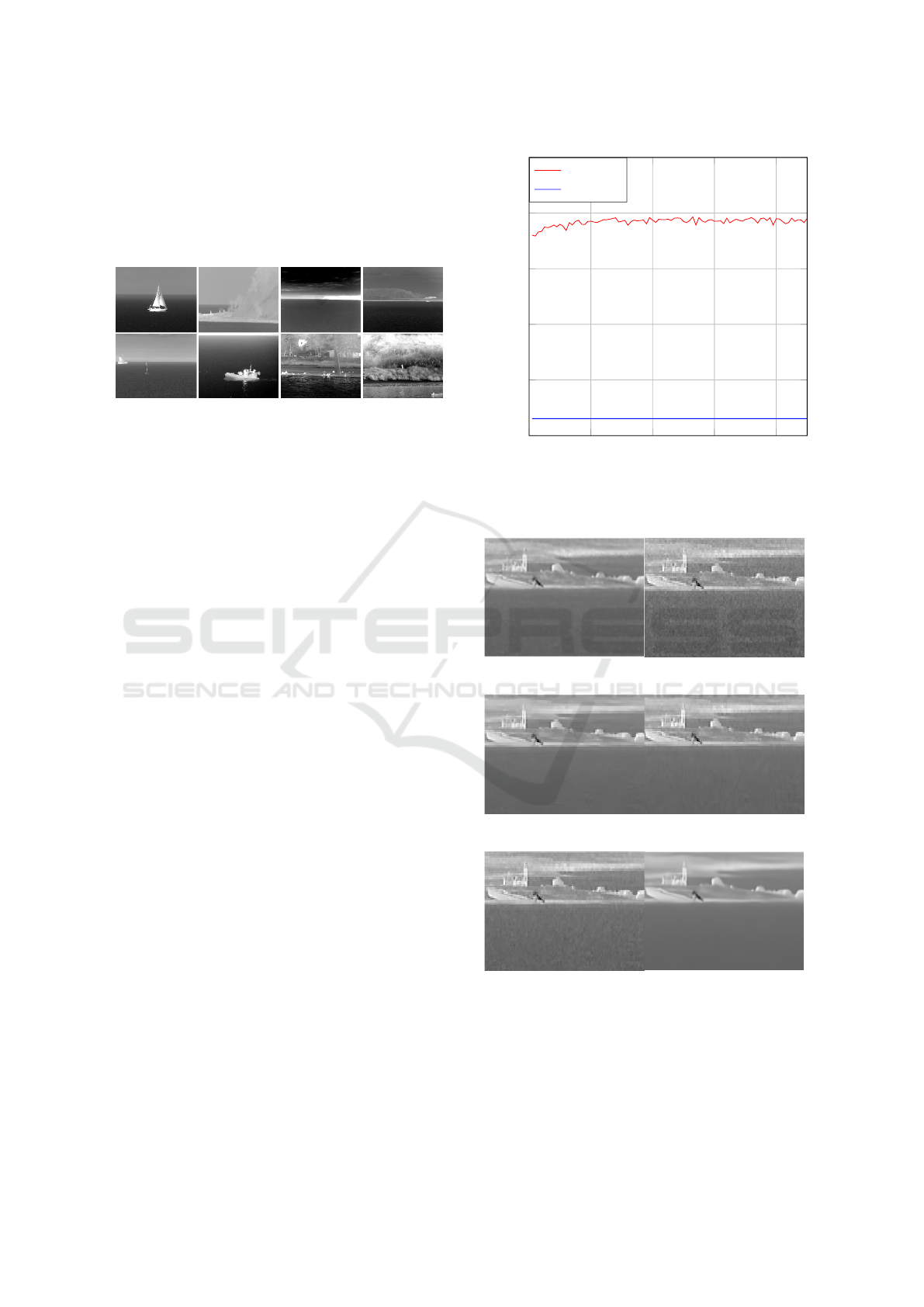
Figure 7: Sample clean images from WTD 71 test dataset.

4.1 Standard Evaluation

The results of the CNNs are evaluated with the stan-

dard peak signal-to-noise ratio (PSNR) and struc-

tural similarity (SSIM) metric and are compared with

the results from a selected number of denoising and

super-resolution methods publicly available for test-

ing. Figure 8 shows the improvement of average

PSNR by our denoising CNN on a batch of the val-

idation data over each training epoch. Denoising is

performed on 44 test images. Figure 9 and Figure 10

show a few denoising examples of granular noise with

BM3D, PGPD, our CNN and DnCNN. The denoising

CNN is not trained to denoise Gaussian noise but is

tested with Gaussian noise of standard deviation (σ)

of 25, to test its robustness. Figure 11 shows an ex-

ample denoising result for Gaussian noise. Each of

the denoising examples show selected areas inside the

original image, while the PSNR values represent the

entire original image. The average performance of

the CNN for both granular noise and Gaussian noise

is shown in Table 3. The results show that the denois-

ing CNN is capable of performing well even without

being explicitly trained for a particular kind of noise

proﬁle. The results also show that the CNN can per-

form well on different noise proﬁles without explicit

manual parameter setup usually required by standard

Gaussian denoisers. In other words, irrespective of

the noise content in terms of the type of noise or the

noise power, the CNN generalizes the denoising prob-

lem well, while other methods need prior information

about the noise for good performance. Another ad-

vantage of the denoising CNN is that it does not de-

grade a clean image or an image with negligible noise

content, when operated on, proving its robustness as

well.

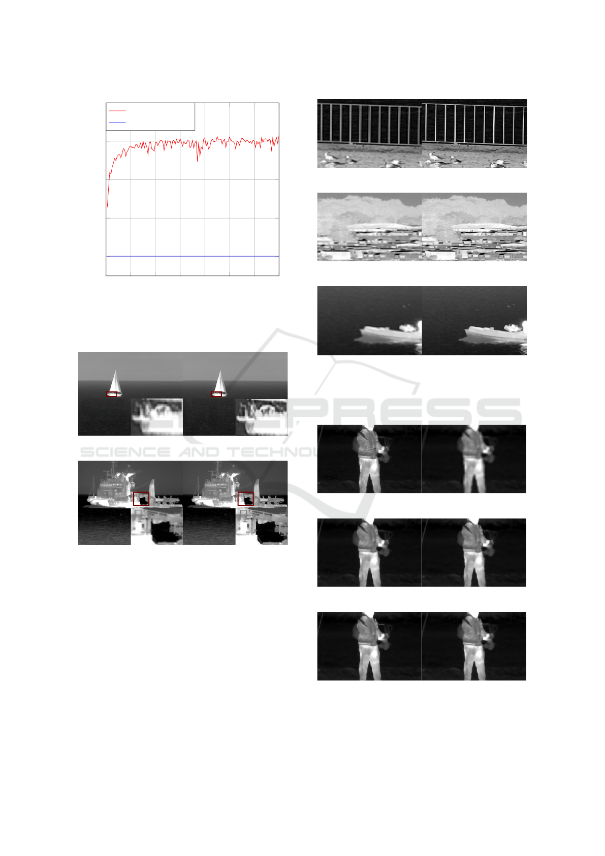
Similar to the denoising CNN, an improvement of

the average PSNR by the super-resolution CNN on a

0 20 40

Epoch

PSNR in dB

denoised

noisy

Figure 8: Comparison of average PSNR of a set of noisy

and denoised validation images at every training epoch.

(a) Original (b) Noisy (33.68 dB)

(e) PGPD (37.95 dB) (f) DnCNN (39.40 dB)

Figure 9: Denoising of granular noise in selected section in

an IR image by different methods.

batch of the validation data over each training epoch,

can be seen in Figure 12. For testing, super-resolution

is performed on the aforementioned test images for

three upsampling ratios. Figure 13 shows two exam-

VISAPP 2018 - International Conference on Computer Vision Theory and Applications

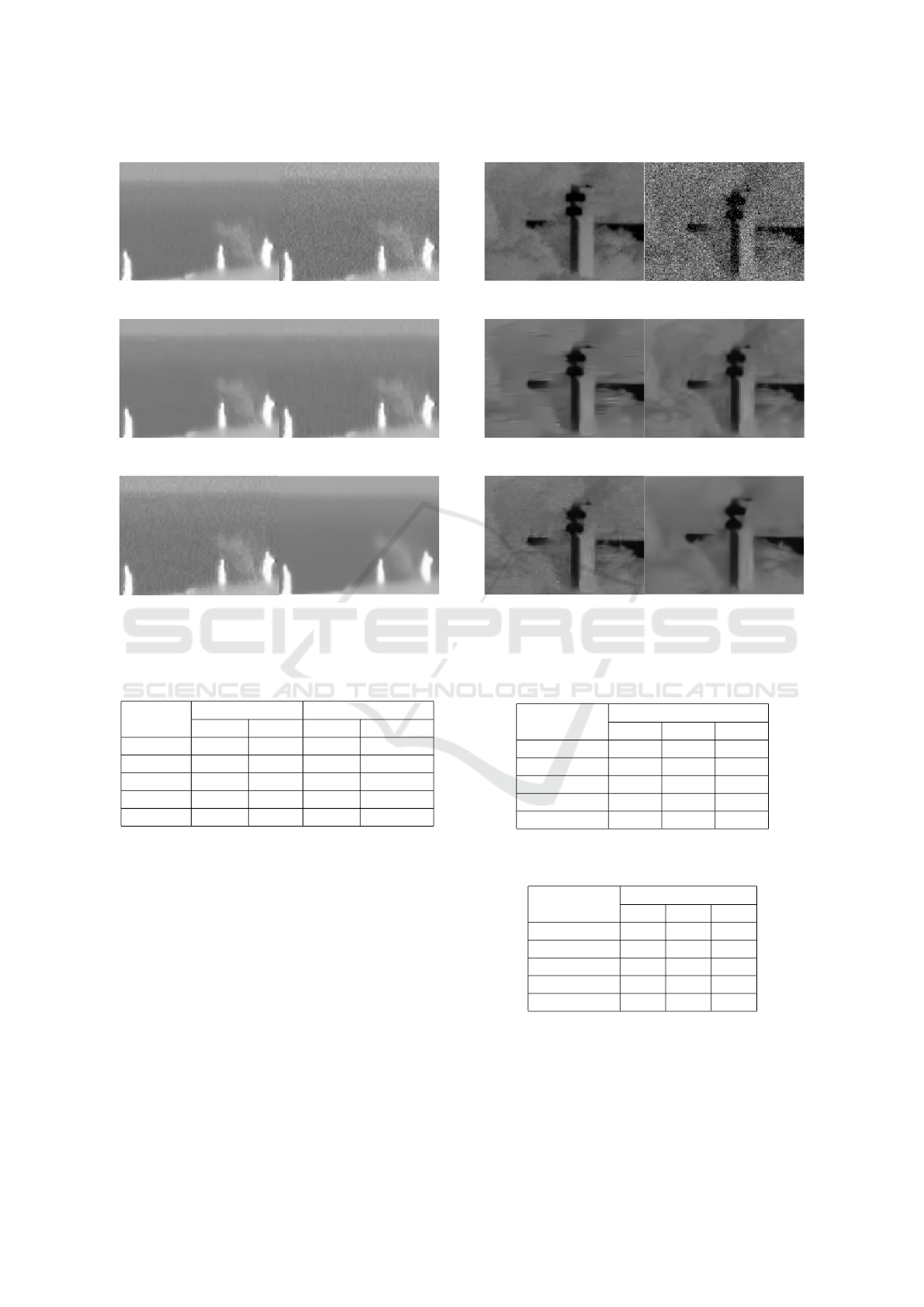
(a) Original (b) Noisy (33.19 dB)

(e) PGPD (38.10 dB) (f) DnCNN (41.65 dB)

Figure 10: Denoising of granular noise in selected section

in an IR image by different methods.

Table 3: Evaluation of average denoising performance

(SSIM, PSNR in dB).

Method

Image Grain Gaussian (σ = 25)

PSNR SSIM PSNR SSIM

None 33.3 0.763 20.58 0.190

CNN 39.47 0.947 33.69 0.841

BM3D 39.42 0.942 33.83 0.848

PGPD 37.47 0.901 32.94 0.802

DnCNN 38.00 0.904 33.99 0.850

ple super-resolution results and Figure 14 shows ex-

ample results for multiple super-resolution factors.

The performance of our super-resolution CNN is also

compared with SRCNN (Dong et al., 2015), DnCNN

(Zhang et al., 2017), and VDSR (Kim et al., 2016),

which are some of the standard state-of-the-art super-

resolution methods. The methods are applied on the

WTD71 dataset and the corresponding results are tab-

ulated in Table 4 and Table 5. Figure 15 shows an ex-

ample from the application of each of these methods

for a super-resolution factor of 4. The results indi-

cate that our CNN is very competitive with respect to

VDSR and DnCNN. Our super-resolution CNN also

has lesser number of training parameters compared to

the other deep networks.

(a) Original (b) Noisy (20.93 dB)

(e) PGPD (31.95 dB) (f) DnCNN (32.05 dB)

Figure 11: Denoising of Gaussian noise (σ=25) in selected

section in an IR image by different methods.

Table 4: Comparison of super-resolution performance

(PSNR).

Method

PSNR (dB)

×2 ×3 ×4

Bicubic 37.25 34.75 33.29

CNN (ours) 39.21 36.15 34.45

SRCNN 38.76 35.91 34.17

VDSR 39.22 36.20 34.54

DnCNN 38.79 36.02 34.45

Table 5: Comparison of super-resolution performance

(SSIM).

Method

SSIM

×2 ×3 ×4

Bicubic 0.92 0.87 0.84

CNN (ours) 0.94 0.90 0.87

SRCNN 0.94 0.89 0.86

VDSR 0.94 0.90 0.88

DnCNN 0.93 0.88 0.85

4.2 Blind Denoising

In real world images, prior knowledge of the degra-

dation is unknown. In this context the test IR images

can only be subjectively evaluated and the improve-

Infrared Image Enhancement in Maritime Environment with Convolutional Neural Networks

0 20 40

80 100 120 140

Epoch

PSNR in dB

super-resolution

bicubic

Figure 12: Comparison of average PSNR of a set of bicubic

and super-resolved (×2) validation images at every training

epoch.

(a) Bicubic (36.06 dB) (b) CNN (Ours) (38.64 dB)

Figure 13: Comparison between bicubic interpolation and

super-resolution (×2) of selected IR images.

ment can be compared through observation. The test

images comprise of 20 IR images corrupted by natu-

ral artefacts. A selection of the original and denoised

image sections are shown in Figure 16. From the ex-

ample images it can be observed that the images con-

tain noise artefacts and the intensity of noise is not

very high. The images are a collection of frames from

speciﬁc videos and have the appearance of graininess

and repetitive patterns. Areas from the original im-

ages and the processed versions of the images in Fig-

ure 16 show the denoising performance of the CNN.

From the images it can be observed that the graininess

(a) Bicubic (23.78 dB) (b) CNN (Ours) (26.73 dB)

(e) Bicubic (29.97 dB) (f) CNN (Ours) (31.28 dB)

Figure 14: Comparison between (a) bicubic and (b) super-

resolution (×2) (c) bicubic and (d) super-resolution (×3)

and (e) bicubic and (f) super-resolution (×4) of selected sec-

tions of IR images.

(a) Original (b) Bicubic (35.07 dB)

(e) VDSR (38.11 dB) (f) DnCNN (38.06 dB)

Figure 15: Super-resolution (×4) of a selected section in an

IR image by different super-resolution methods.

VISAPP 2018 - International Conference on Computer Vision Theory and Applications

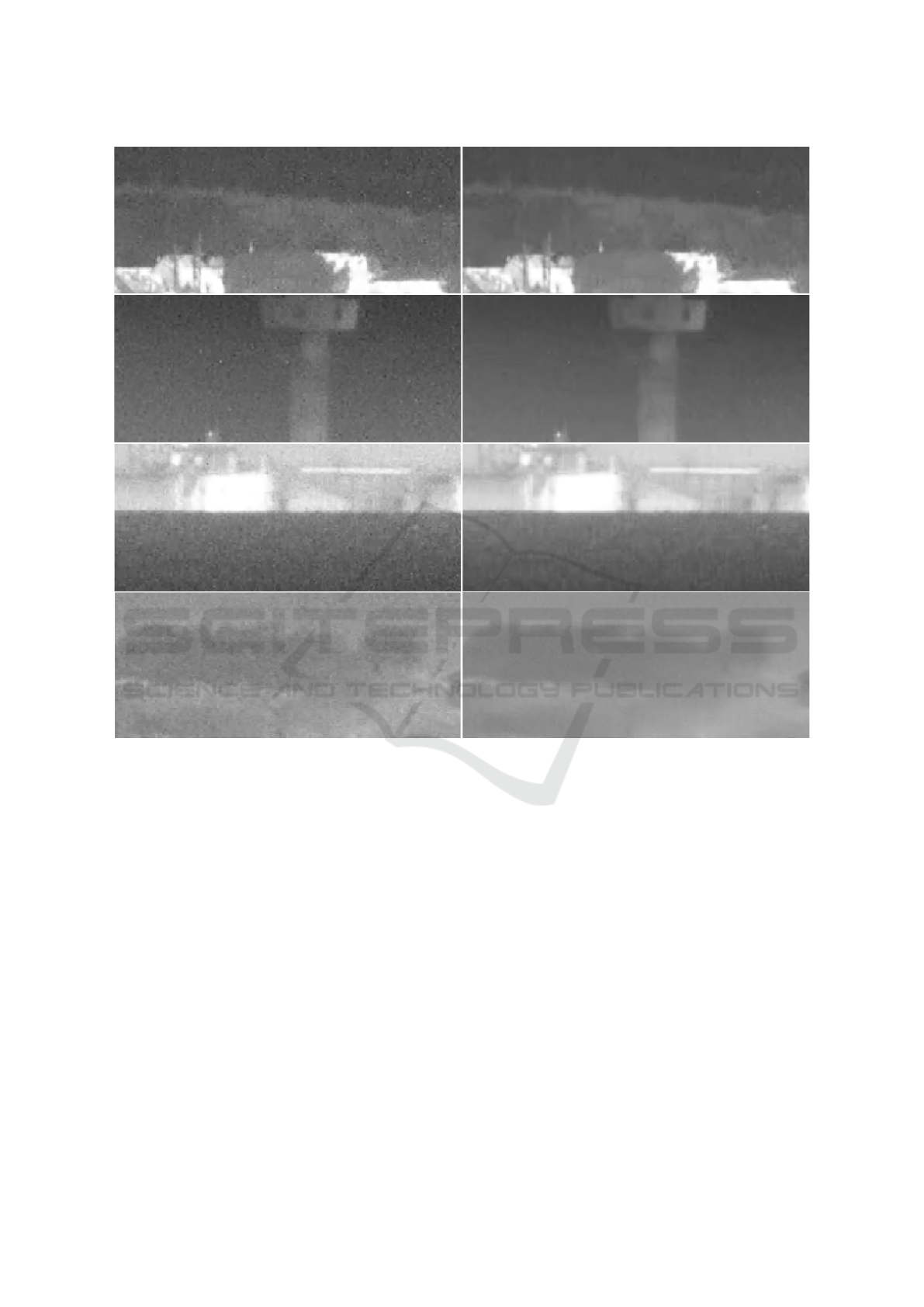
Figure 16: Example of denoising of natural images with original image areas shown in the left column and the corresponding

denoised areas shown in the right column (best observed on a monitor).

of the images is reduced while preserving the edges

considerably well. The differences are best observed

on a monitor.

5 CONCLUSION

In this paper we have proposed image enhancement

approaches for maritime IR images. We use two

CNNs with residual architectures based on regression

losses to denoise and super-resolve IR images. The

training images are created by adding noise content in

clean images. From the objective and subjective eval-

uation based on example images it can be concluded

that the denoising and super-resolution performs well

with our networks. The results show that the CNNs

are able to improve the quality of IR images. The

results also encourage further investigation of simple

CNN structures and improving their robustness to dif-

ferent types of noise, different intensities of noise and

different grain sizes since the present network is lim-

ited to the data it is trained with. Further investigation

can be made on the training data requirement, e.g.,

training with thermal images only, for better domain

speciﬁc learning. It is also noteworthy that other vi-

sion tasks like segmentation, detection, and stabiliza-

tion also beneﬁt from the enhancement of images and

the inﬂuence can be investigated in the future.

REFERENCES

Brown, M. and S

usstrunk, S. (2011). Multispec-

tral SIFT for scene category recognition. In

Computer Vision and Pattern Recognition

(CVPR11), 177-184, Colorado Springs. IEEE.

Infrared Image Enhancement in Maritime Environment with Convolutional Neural Networks

doi:10.1109/CVPR.2011.5995637. Retrieved from

http://ivrl.epﬂ.ch/supplementary material/cvpr11/.

Burger, H. C., Schuler, C. J., and Harmeling, S. (2012).

Image denoising: Can plain neural networks compete

with BM3D? In IEEE Conference on Computer Vi-

sion and Pattern Recognition, 2392-2399. IEEE. doi:

10.1109/CVPR.2012.6247952.

Dabov, K., Foi, A., Katkovnik, V., and Egiazarian, K.

(2007). Image denoising by sparse 3-d transform-

domain collaborative ﬁltering. In IEEE Transac-

tions on Image Processing, 16(8), 2080-2095. IEEE.

doi:10.1109/TIP.2007.901238.

Dong, C., Loy, C. C., He, K., and Tang, X. (2015). Im-

age super-resolution using deep convolutional net-

works. In IEEE Transactions on Pattern Analy-

sis and Machine Intelligence, 38(2), 295-307. IEEE.

doi:10.1109/TPAMI.2015.2439281.

Elad, M. and Aharon, M. (2006). Image denoising via

learned dictionaries and sparse representation. In

IEEE Computer Society Conference on Computer Vi-

sion and Pattern Recognition (CVPR), 1, 895-900.

IEEE. doi:10.1109/CVPR.2006.142.

Glorot, X. and Bengio, Y. (2010). Understanding the

difﬁculty of training deep feedforward neural net-

works. In Proceedings of the Thirteenth Inter-

national Conference on Artiﬁcial Intelligence and

Statistics, 9, 249-256. JMLR. Retrieved from

http://proceedings.mlr.press/v9/glorot10a.html.

Goldstein, T. and Osher, S. (2009). The split breg-

man method for L1 regularized problems. In SIAM

Journal on Imaging Sciences, 2(2), 323-343. Society

for Industrial and Applied Mathematics Philadelphia.

doi:10.1137/080725891.

He, K., Zhang, X., Ren, S., and Sun, J. (2016). Deep

residual learning for image recognition. In IEEE Con-

ference on Computer Vision and Pattern Recognition

(CVPR), 770-778. IEEE. doi:10.1109/CVPR.2016.90.

Jain, V. and Seung, S. (2009). Natural image de-

noising with convolutional networks. In Ad-

vances in Neural Information Processing Systems

21, 769-776. Curran Associates, Inc. Retrieved

from http://papers.nips.cc/paper/3506-natural-image-

denoising-with-convolutional-networks.pdf.

J.Xu, L.Zhang, Zuo, W., Zhang, D., and Feng, X. (2015).

Patch group based nonlocal self-similarity prior learn-

ing for image denoising. In IEEE International Con-

ference on Computer Vision (ICCV), 244-252. IEEE.

doi:10.1109/ICCV.2015.36.

Kim, J., Lee, J. K., and Lee, K. M. (2016). Accurate

image super-resolution using very deep convolutional

networks. In IEEE Computer Society Conference on

Computer Vision and Pattern Recognition (CVPR),

1646-1654. IEEE. doi:10.1109/CVPR.2016.182.

Kingma, D. P. and Ba, J. (2014). Adam: A method for

stochastic optimization. In 3rd International Confer-

ence for Learning Representations. CoRR. Retrieved

from http://arxiv.org/abs/1412.6980.

Micchelli, C. A., Shen, L., and Y.Xu (2011). Prox-

imity algorithms for image models: denoising.

In Inverse Problems, 27(4). Retrieved from

http://stacks.iop.org/0266-5611/27/i=4/a=045009.

Pan, T., Zhongliang, F., Lili, W., and Kai, Z. (2016).

Perceptual loss with fully convolutional for image

residual denoising. In T. Tan et al. (eds.) Chinese

Conference on Pattern Recognition (CCPR), 122-132.

Springer. Retrieved from https://doi.org/10.1007/978-

981-10-3005-5 11.

Vedaldi, A. and Lenc, K. (2015). Matconvnet: Con-

volutional neural networks for matlab. In Pro-

ceedings of the 23rd ACM international confer-

ence on Multimedia. CoRR. Retrieved from

http://arxiv.org/abs/1412.4564.

Zhang, K., Zuo, W., Chen, Y., Meng, D., and Zhang, L.

(2017). Beyond a gaussian denoiser: Residual learn-

ing of deep cnn for image denoising. In IEEE Transac-

tions on Image Processing, 26(7), 3142-3155. IEEE.

doi:10.1109/TIP.2017.2662206.

Zhang, Z. M., Tsai, B. K., and G.Machin (2010). Radiomet-

ric Temperature Measurements. Elsevier, 1st edition.

Zhou, Z., Cao, J., and Liu, W. (2009). Contourlet-

based image denoising algorithm using adaptive win-

dows. In 4th IEEE Conference on Industrial Elec-

tronics and Applications (ICIEA), 3654-3657. IEEE.

doi:10.1109/ICIEA.2009.5138888.

VISAPP 2018 - International Conference on Computer Vision Theory and Applications