
Deep Learning for 3D Shape Classification based on Volumetric Density
and Surface Approximation Clues
Ludovico Minto, Pietro Zanuttigh and Giampaolo Pagnutti
Department of Information Engineering, University of Padova, Via Gradenigo 6B, Padova, Italy
Keywords:
3D Shapes, Classification, Deep Learning, NURBS.
Abstract:
This paper proposes a novel approach for the classification of 3D shapes exploiting surface and volumetric
clues inside a deep learning framework. The proposed algorithm uses three different data representations. The
first is a set of depth maps obtained by rendering the 3D object. The second is a novel volumetric representation
obtained by counting the number of filled voxels along each direction. Finally NURBS surfaces are fitted over
the 3D object and surface curvature parameters are selected as the third representation. All the three data
representations are fed to a multi-branch Convolutional Neural Network. Each branch processes a different
data source and produces a feature vector by using convolutional layers of progressively reduced resolution.
The extracted feature vectors are fed to a linear classifier that combines the outputs in order to get the final
predictions. Experimental results on the ModelNet dataset show that the proposed approach is able to obtain
a state-of-the-art performance.
1 INTRODUCTION
The recent introduction of consumer depth cameras
has made 3D data acquisition easier and widely in-
creased the interest in methods for the automatic clas-
sification and recognition of 3D shapes. This has been
a long term research task, however algorithms dealing
with this problem have achieved a completely satis-
factory performance only recently, specially thanks to
the introduction of deep learning techniques.
Differently from standard images, that can be
straightforward sent to Convolutional Neural Net-
works (CNN), the processing of 3D point clouds with
deep learning techniques requires first of all to rep-
resent the data into a form that is suitable for the
deep learning algorithms. This work proposes a novel
method for the classification of 3D shapes based on
the idea of representing the data with multiple 2D
structures and then exploiting a multi-branch CNN.
We propose to use three different representations. The
first, that we derived from the approach presented in
(Zanuttigh and Minto, 2017), is given by a set of
different depth maps obtained by rendering the in-
put shape from six different viewpoints, which is a
quite standard approach. The second representation
is a novel volumetric descriptor that captures the den-
sity, i.e., the amount of filled voxels, along directions
parallel to the 3D axes. Finally, we also fit parametric
Non-Uniform Rational B-Spline (NURBS) surfaces
on the objects and calculate the two principal curva-
tures at each surface location, obtaining 2D maps that
describe the local curvature of the shape.
The three representations are used as input for
the neural network: the CNN has 15 branches, each
branch analyzing a different data source. Specifically,
there are 6 branches for the depth maps, 3 for the
volumetric data and finally 6 for the curvature data.
Each branch contains 4 (for depth and surface data)
or 5 (for the volumetric densities) layers that progres-
sively reduce the resolution until a single feature vec-
tor is obtained for each of them. In order to reduce
the complexity, we also share the weights by dividing
the depth and curvature branches in two groups, one
containing the four side views and one for the top and
bottom views. Finally, the feature vectors are concate-
nated into a single vector which is fed to a softmax
classifier that produces the shape classification.
The paper starts by presenting the related works in
Section 2. Then Section 3 presents the proposed data
representation. Section 4 describes the deep learning
network. Finally the results are discussed in Section
5 while Section 6 draws the conclusions.
Minto, L., Zanuttigh, P. and Pagnutti, G.
Deep Learning for 3D Shape Classification based on Volumetric Density and Surface Approximation Clues.
DOI: 10.5220/0006619103170324
In Proceedings of the 13th International Joint Conference on Computer Vision, Imaging and Computer Graphics Theory and Applications (VISIGRAPP 2018) - Volume 5: VISAPP, pages
317-324
ISBN: 978-989-758-290-5
Copyright © 2018 by SCITEPRESS – Science and Technology Publications, Lda. All rights reserved
317

2 RELATED WORKS
The retrieval and classification of 3D shapes is a long
term research field. Many different schemes based
on global representations and local shape descriptors
have been proposed in the past. For an overview
of the field see review papers like (Tangelder and
Veltkamp, 2004; Guo et al., 2014; Li et al., 2015). As
for many other classification tasks, the introduction
of deep learning approaches has allowed large im-
provements and completely changed the way of deal-
ing with this problem. Several different deep learn-
ing techniques and in particular Convolutional Neu-
ral Networks (CNN) have been proposed. The funda-
mental issue in these methods is that 3D representa-
tions do not lay on a regular structure as 2D images,
making it necessary to convert the data into a repre-
sentation suitable for the network structure or to adapt
the network model.
A first family of approaches is based on the idea
of rendering the 3D model from different viewpoints
and then use the obtained silhouettes, images or depth
maps as input to a standard convolutional network.
The work of (Sinha et al., 2016) exploits a spherical
parametrization to represent the mesh in a geometry
image containing curvature information that is fed to
a CNN. The method of (Shi et al., 2015) exploits the
idea of representing the 3D object with a panoramic
view and uses an ad-hoc CNN structure for this kind
of images. In the scheme of (Johns et al., 2016) pairs
of views of the object are used together with a second
CNN for the selection of the best viewpoints. Another
approach exploiting this strategy is (Su et al., 2015)
that extracts a set of color views from the 3D model
and combines the information into a single shape de-
scriptor using a CNN architecture. Multiple depth
maps rendered from the object have been exploited
in (Zanuttigh and Minto, 2017), which we take as a
starting point for the depth-based component of the
proposed method.
A second possibility is to use volumetric repre-
sentations instead, together with three-dimensional
CNNs applied on the voxel structure. In (Wu et al.,
2015) a Convolutional Deep Belief Network is ex-
ploited to represent input shapes as probability dis-
tributions on a 3D voxel grid. A highly performing
method based on the voxel representation is (Brock
et al., 2016), which exploits a variation of the ResNet
architecture. In the PointNet approach (Garcia-Garcia
et al., 2016) density occupancy grids are fed as input
to a CNN for 3D shape classification. The approach
of (Maturana and Scherer, 2015) relies on a 3D CNN
fed with volumetric occupancy grids while (Wu et al.,
2016) jointly exploits Volumetric Convolutional Net-
Figure 1: Example of the six depth maps used for the anal-
ysis of a chair 3D model. Notice how there are four similar
side views (blue boxes) and the top and bottom ones (orange
boxes).
works and Generative Adversarial Networks. A com-
parison between the volumetric and the multi-view
scheme is presented in (Qi et al., 2016), also propos-
ing various improvements to both approaches.
Finally, some approaches exploit non-standard
deep learning architectures in order to deal with un-
structured data. The approach of (Li et al., 2016) ex-
ploits field probing filters to extract the features and
optimizes not only the weights of the filters as in stan-
dard CNNs but also their locations. Another scheme
of this family is the one of (Klokov and Lempitsky,
2017), which presents a deep learning architecture
suited for the Kd-tree representation of volumetric
data. A deep network able to directly process point
cloud data has been presented in (Qi et al., 2017).
3 SURFACE AND VOLUME
REPRESENTATION FOR DEEP
LEARNING
The proposed algorithm works in two stages: a pre-
processing step that constructs the input data fol-
lowed by a multi-branch Convolutional Neural Net-
work (CNN) that performs the classification. The pro-
posed data representation is described in this section
while the CNN architecture will be the subject of Sec-
tion 4. In this work we consider three different data
representations:
1. A multi-view representation made of a set of six
depth maps extracted from the 3D model.
2. A volumetric representation obtained by measur-
ing the number of filled voxels along directions
parallel to the 3D space axes.
3. A surface representation given by the curvatures
of NURBS surfaces fitted over the 3D model.
VISAPP 2018 - International Conference on Computer Vision Theory and Applications
318
(a) (b) (c)
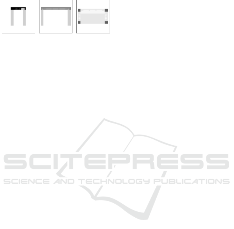
Figure 2: Example of the three voxel density maps for a
table 3D model, computed along the x-axis (a), y-axis (b)
and z-axis (c) respectively.
3.1 Multi-view Representation
In order to build this representation, we first compute
the bounding box of the input 3D model. Then the 3D
model is rendered from six different viewpoints, each
corresponding to one of the six faces of the bounding
box. For each of the six views we extract the depth
information from the z-buffer, thus obtaining six dif-
ferent depth maps for each object (see Fig. 1). The
output depths have a resolution of 320 × 320 pixels
which, in our experiments, proved to be a reason-
able trade-off between the accuracy of the represen-
tation and the computational effort required to train
the neural network. The six depth maps represent the
input for the proposed classifier. Their usage makes
it possible to capture a complete description of the
3D shape without considering a full volumetric struc-
ture that would require a larger amount of data due
to the higher dimensionality. Furthermore, the depth
map conveys a greater information content if com-
pared with the silhouettes of the shape. Notice that,
assuming the object is lying on the ground, the six
views can be divided into four side views with a sim-
ilar structure and the bottom and top views. Indeed,
for many real world objects it is reasonable to assume
they can rotate around the vertical axis while being
constrained to lay on the ground. Moreover, the fact
that typically the four side views have a similar con-
tent while the top and bottom capture a different rep-
resentation will be exploited in the construction of the
neural network. In order to improve the robustness of
the proposed approach with respect to rotations, we
also considered the option of augmenting the train-
ing dataset by creating randomly rotated copies of the
3D models, however this did not lead to accuracy im-
provements on the considered experimental dataset.
We disabled this option since it was also leading to an
increase in the training time due to the larger dataset
size. However this step can be adopted in order to
deal with more generic datasets.
Finally, local contrast normalization is applied to
each input depth map independently.
3.2 Volume Representation
Volumetric representations have been exploited in
various 3D classification schemes like the ones of
(Wu et al., 2015; Wu et al., 2016; Maturana and
Scherer, 2015). Unfortunately, the performance of ap-
proaches exploiting the full volumetric representation
is affected by the fact that the 3D structure containing
the voxel data uses a considerable amount of mem-
ory and requires 3D convolutional filters with a higher
number of parameters. The increased dimensional-
ity and requirements are typically compensated by us-
ing low resolution and simpler networks, but this also
impacts on the performance. In order to exploit the
information given by the volumetric data and at the
same time preserve the simpler and faster operations
of 2D representations we introduce a novel data rep-
resentation. The idea is to build a set of three density
maps representing the density of filled voxels along
the directions corresponding to each of the three axes.
More in detail, the x-axis representation is built by
quantizing the yz-plane into 32 × 32 cells and count-
ing how many filled voxels are encountered by going
down along the x-axis from each location (i.e., letting
x vary after fixing the value of the y and z coordi-
nates). The representation for the y-axis and z-axis
are built in the same way by swapping the axes (i.e.,
fix x and z and let y vary or fix x and y and let z vary).
A visual example on a table model is shown in Fig.
2. Notice how, for example, the z profile (i.e., top
profile) captures the table surface (low density) and
four high density spots corresponding to the four legs
of the table. Finally, as for depth information, local
contrast normalization has been applied to the data.
3.3 Surface Representation
The third data representation is based on geometric
properties of parametric surfaces that approximate the
objects shape. The idea is to consider the six views of
the first representation and to obtain a Non-Uniform
Rational B-Spline (NURBS) fitting surface for each
of them. In order to perform this task, we consider the
3D points corresponding to each depth sample and we
approximate them with a continuous parametric sur-
face S(u, v), computed by solving an over-determined
system of linear equations in the least-squares sense.
Notice that the u, v parametric range of the NURBS
surface corresponds to the rectangular grid structure
of the depth map. The NURBS degrees in the u and
v directions have been set to 3, while the weights are
all equal to 1, i.e., our fitted surfaces are non-rational
(splines). We used the surface fitting algorithm pre-
sented in (Pagnutti and Zanuttigh, 2016; Minto et al.,
Deep Learning for 3D Shape Classification based on Volumetric Density and Surface Approximation Clues
319
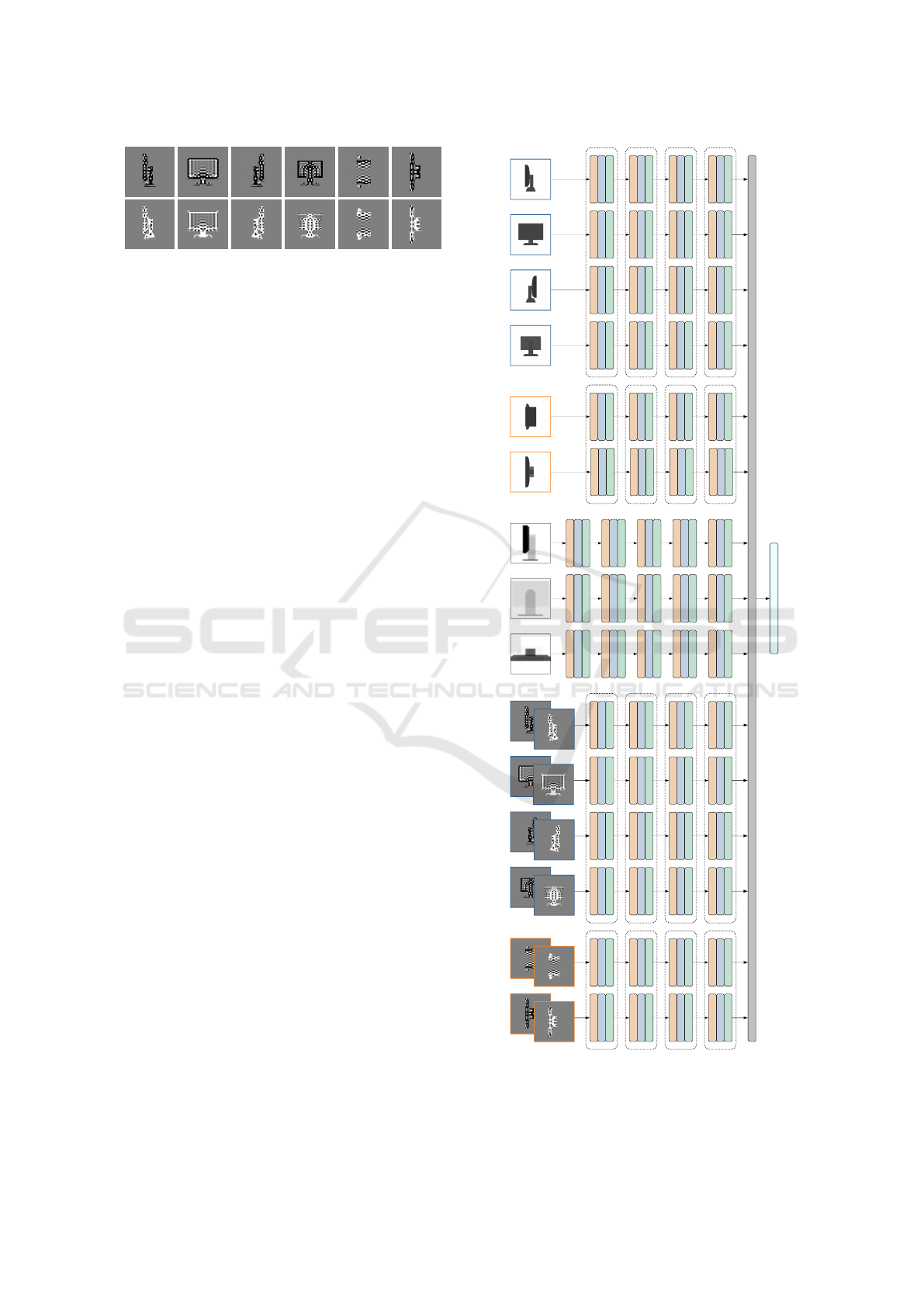
Figure 3: Example of curvature maps for a 3D model of the
monitor class. The first row shows the k
1
curvature maps for
the six views, while the second row shows the data relative
to k
2
. The data have been scaled for visualization purposes
(dark colors correspond to negative values and bright colors
to positive ones).
2016), see these publications for more details on this
task. Notice how the usage of NURBS surfaces pro-
vides a geometric model that is well suitable to de-
scribe arbitrary shapes, not only planar ones. After
fitting the surfaces we determine their two principal
curvatures k
1
and k
2
at each sample location. An ex-
ample of the resulting information is visible in Fig. 3,
that shows the two curvature maps for a sample ob-
ject. These data are locally normalized and then used
as the last input for the CNN classifier.
4 DEEP NETWORK
ARCHITECTURE
The proposed classifier takes in input the three rep-
resentations and gives in output a semantic label for
each scene. For this task an ad-hoc Convolutional
Neural Network (CNN) architecture with multiple
branches has been developed. The structure of the
network is summarized in Fig. 4. It is made of two
main parts, namely a set of branches containing con-
volutional layers and a linear classification stage com-
bining the information from the different branches.
The network has been designed in order to pro-
duce a single reliable classification output for each
3D object starting from the multi-modal input of Sec-
tion 3. Its structure stems from the semantic segmen-
tation architectures of (Farabet et al., 2013; Couprie
et al., 2013; Minto et al., 2016), but greatly differs
from them due to the different task and the particular
nature of the exploited data.
In the first part there are 15 different branches, di-
vided in 3 groups (see Fig. 4 and Table 1). The first
group has 6 branches and processes the depth infor-
mation. Each branch takes in input a single depth map
at the resolution of 320 × 320 pixels and extracts a
feature vector for the input by applying a sequence of
convolutional layers. More in detail, each branch has
4 convolutional layers (CONV), each followed by a
rectified linear unit activation function (RELU) and a
max-pooling layer (MAXP). The first layer has 48 fil-
320x240x3
h1h2a
320x240x3
h1h2a
CONV 3x3
RELU
MAXP (4,4)
320x240x3
h1h2a
320x240x3
fc1c2
320x240x3
h1h2a
320x240x3
fc1c2
CONCATENATE
CONV 3x3
RELU
MAXP (4,4)
CONV 3x3
RELU
MAXP (4,4)
CONV 3x3
RELU
MAXP (5,5)
CONV 3x3
RELU
MAXP (4,4)
CONV 3x3
RELU
MAXP (4,4)
CONV 3x3
RELU
MAXP (4,4)
CONV 3x3
RELU
MAXP (5,5)
CONV 3x3
RELU
MAXP (4,4)
CONV 3x3
RELU
MAXP (4,4)
CONV 3x3
RELU
MAXP (4,4)
CONV 3x3
RELU
MAXP (5,5)
CONV 3x3
RELU
MAXP (4,4)
CONV 3x3
RELU
MAXP (4,4)
CONV 3x3
RELU
MAXP (4,4)
CONV 3x3
RELU
MAXP (5,5)
CONV 3x3
RELU
MAXP (4,4)
CONV 3x3
RELU
MAXP (4,4)
CONV 3x3
RELU
MAXP (4,4)
CONV 3x3
RELU
MAXP (5,5)
CONV 3x3
RELU
MAXP (4,4)
CONV 3x3
RELU
MAXP (4,4)
CONV 3x3
RELU
MAXP (4,4)
CONV 3x3
RELU
MAXP (5,5)
CONV 3x3
RELU
MAXP (2,2)
CONV 3x3
RELU
MAXP (2,2)
CONV 3x3
RELU
MAXP (2,2)
CONV 3x3
RELU
MAXP (2,2)
CONV 3x3
RELU
MAXP (2,2)
CONV 3x3
RELU
MAXP (4,4)
CONV 3x3
RELU
MAXP (4,4)
CONV 3x3
RELU
MAXP (4,4)
CONV 3x3
RELU
MAXP (5,5)
CONV 3x3
RELU
MAXP (4,4)
CONV 3x3
RELU
MAXP (4,4)
CONV 3x3
RELU
MAXP (4,4)
CONV 3x3
RELU
MAXP (5,5)
CONV 3x3
RELU
MAXP (4,4)
CONV 3x3
RELU
MAXP (4,4)
CONV 3x3
RELU
MAXP (4,4)
CONV 3x3
RELU
MAXP (5,5)
CONV 3x3
RELU
MAXP (4,4)
CONV 3x3
RELU
MAXP (4,4)
CONV 3x3
RELU
MAXP (4,4)
CONV 3x3
RELU
MAXP (5,5)
CONV 3x3
RELU
MAXP (4,4)
CONV 3x3
RELU
MAXP (4,4)
CONV 3x3
RELU
MAXP (4,4)
CONV 3x3
RELU
MAXP (5,5)
CONV 3x3
RELU
MAXP (4,4)
CONV 3x3
RELU
MAXP (4,4)
CONV 3x3
RELU
MAXP (4,4)
CONV 3x3
RELU
MAXP (5,5)
CONV 3x3
RELU
MAXP (2,2)
CONV 3x3
RELU
MAXP (2,2)
CONV 3x3
RELU
MAXP (2,2)
CONV 3x3
RELU
MAXP (2,2)
CONV 3x3
RELU
MAXP (2,2)
CONV 3x3
RELU
MAXP (2,2)
CONV 3x3
RELU
MAXP (2,2)
CONV 3x3
RELU
MAXP (2,2)
CONV 3x3
RELU
MAXP (2,2)
CONV 3x3
RELU
MAXP (2,2)
SOFTMAX CLASSIFIER
Figure 4: Layout of the proposed multi-branch Convolu-
tional Neural Network (the dashed boxes enclose layers
sharing the same weights).
VISAPP 2018 - International Conference on Computer Vision Theory and Applications
320
ters while the second, third and fourth ones have 128
filters, all being 3 × 3 pixels wide. The max-pooling
stages subsample the data by a factor of 4 in each di-
mension in the first three stages and of 5 in the last
one. Thanks to this approach the full resolution is
used only in the first layer, while it is progressively
reduced in the next ones until a single classification
hypothesis is obtained for the whole depth map in
the last layer. The computational resources required
for the training are decreased as a consequence, since
in the inner layers the resolution is strongly reduced.
The final output is a 128-elements vector for each
depth map.
Concerning the weights of the convolutional fil-
ters there are two approaches commonly used. The
first is to have independent weights for each branch
of the network. This better adapts the network to
the various views, however it leads to a large amount
of parameters thus increasing the computational com-
plexity and the risk of over-fitting. Furthermore, this
makes also the approach more dependent on the pose
of the model since, changing the pose, data can move
from one view to another. Other approaches share the
weights across the various branches (Farabet et al.,
2013; Couprie et al., 2013), thus reducing the com-
plexity but also the discrimination capabilities of the
network. A key observation is that the captured data
are typically similar in the four side views but differ-
ent for the top and bottom ones. Thus we decided
to use a hybrid solution between the two approaches
with a shared set of weights for the four side views
and a different set for the top and bottom ones. This
proved to be a good trade-off between the two solu-
tions, providing a good accuracy with a reasonable
training time and a partial invariance at least to the ro-
tation along the vertical axis. Notice that the approach
assumes that the objects are laying on the ground in
order to distinguish between the side and top or bot-
tom views, however this is a reasonable assumption
for most real world objects.
The branches in the second set deal with volumet-
ric data. In this case there are 3 branches, associated
to the x-axis, y-axis and z-axis respectively. The input
data have a lower resolution, namely 32 × 32 pixels
(see Section 3.2 for the rationale behind this choice).
Each branch has 5 convolutional layers, each one with
a RELU activation and a max-pooling stage. There
are 48 convolutional filters in the first layer and 128
in the other ones. The filters are still 3 × 3, however
this time the max-pooling stages subsample the data
by a factor of 2 due to the lower starting resolution.
In this case weights are independent for each branch
since the three profiles capture different data. Notice
also that, given the low resolution, sharing the weights
Table 1: Summary of the properties of the various layers in
the Convolutional Neural Network.
Depth and NURBS Volumetric
# Filt. Pool Res. # Filt. Pool Res.
L1 48 4×4 320×320 48 2×2 32×32
L2 128 4×4 80×80 128 2×2 16×16
L3 128 4×4 20×20 128 2×2 8×8
L4 128 5×5 5×5 128 2×2 4×4
L5 - - - 128 2×2 2×2
among the three branches would not bring any sub-
stantial reduction in the training effort.
Finally, the branches of the third set process the
surface fitting data. There is a set of coefficients con-
tained in a 2-channel 320 × 320 pixels map for each
3D view, the structure being very similar to the one of
first group. In this case, there are two channels cor-
responding to the two principal curvatures instead of
one only. Aside from this, the network architecture is
exactly the same as in the first group.
The 128-elements feature vectors produced by
each one of the 15 channels are then concatenated in
a 15 × 128 = 1920 elements vector and fed to a final
softmax classifier with a 1920 × n
c
weight matrix and
no bias, where n
c
is the considered number of classes.
We set n
c
equal to 10 and 40 depending on the dataset
used for experimental results.
The network is trained as described in Section 5
to produce a labeling of each 3D shape by assign-
ing it one out of the n
c
different categories. To this
aim, a multi-class cross-entropy loss function is mini-
mized throughout the training process. We set a limit
of 100 epochs, even if the optimal solution is typically
reached earlier.
5 EXPERIMENTAL RESULTS
We evaluated the performance of the proposed ap-
proach on the large-scale Princeton ModelNet dataset
(Wu et al., 2015), containing 3D object models along
with their ground-truth categories. We present our re-
sults both for the 10-class ModelNet10 subset and for
the larger 40-class ModelNet40 subset. In particular,
we trained and tested the network described in Section
4 on the two subsets independently. We adopted the
standard training and test splits as provided along with
each subset data. Specifically, for our results on the
ModelNet10 subset we trained the network on 3991
samples, leaving aside 908 samples for the test. As
to the ModelNet40 subset, we performed the training
and testing using 9843 and 2468 samples respectively.
In both cases the training has been carried out by
Deep Learning for 3D Shape Classification based on Volumetric Density and Surface Approximation Clues
321
minimizing a multi-class cross-entropy loss function
with the Stochastic Gradient Descent (SGD) algo-
rithm. We used the Theano framework (Theano De-
velopment Team, 2016) for the implementation.
Starting from the ModelNet10 subset, we first
evaluate the impact of each one of the three data rep-
resentations separately. The results reported in Ta-
ble 2 suggest that the depth maps extracted from the
3D model rendering carry the largest information con-
tent, achieving an average accuracy of 93.2% when
used alone. A remarkable accuracy can also be ob-
tained by feeding the CNN with volumetric profiles
only, correctly predicting 91.2% of the models in the
test set. Despite this value is lower than the one de-
rived using depth data, it is still noteworthy that it has
been obtained with a low resolution data representa-
tion (32 × 32 pixels). Even if volumetric profiles size
equal to just 1% of depth data, results demonstrate
that it is still possible to correctly classify most of
the 3D models using this representation alone. Fi-
nally, the accuracy obtained using only NURBS sur-
face curvature data is 90.9%, lower than the other two
descriptors but still noticeable, proving also the effec-
tiveness of this representation. By combining all the
three representations together we achieved an average
accuracy of 93.6% on the test set, higher than the one
obtained by taking each representation separately.
An in-depth analysis of the performance is shown
in Table 3, which contains the confusion matrix of the
proposed approach on the ModelNet10 dataset.
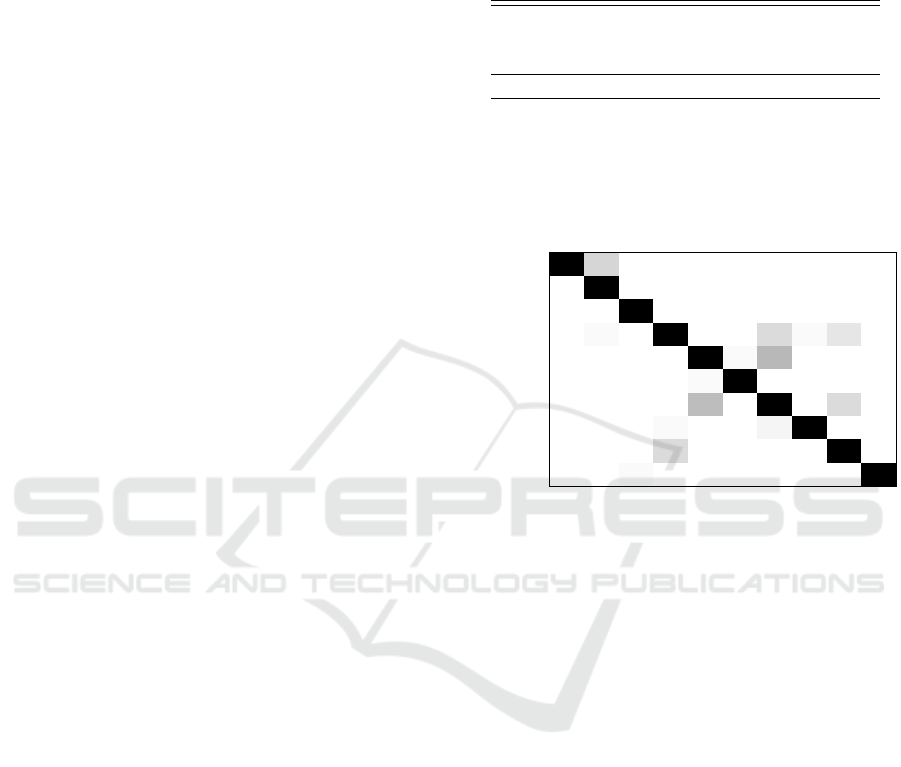
Notice how the proposed method is able to achieve
a very high accuracy on most classes. Some of them
are almost perfectly recognized, e.g. the bed, chair,
monitor and toilet classes. On the other side, some
critical situations also exist such as the confusion be-
tween the night stand and dresser classes, an expected
issue since these two classes have similar shapes and
the disambiguation is difficult in some samples even
for a human observer. Another challenging recogni-
tion task is to distinguish between the table and desk
classes, since in most cases the objects share a simi-
lar structure with a flat surface supported by the legs.
Nonetheless, most samples in these classes are cor-
rectly recognized even if some errors are present.
The performance of our approach has also
been compared with some recent state-of-the-art ap-
proaches on the ModelNet10 dataset. The comparison
is reported in Table 4: the average accuracy of 93.6%
obtained by combining all three data representations
is higher than most of previous works. Specifically,
only (Brock et al., 2016) and (Klokov and Lempitsky,
2017) outperform our approach, the second one by a
limited performance gap.
The approach has been evaluated also on the larger
Table 2: Average accuracies on the ModelNet10 and Mod-
elNet40 datasets for the proposed method when using the
three different data representations taken separately as well
as their combination.
Approach ModelNet10 ModelNet40
Depth maps 93.2% 88.0%
Volumetric 91.2% 86.9%
NURBS 90.9% 85.2%
Combined 93.6% 89.3%
Table 3: Confusion matrix for the proposed approach on the
ModelNet10 dataset. Values are given in percentage.
bathtub
bed
chair
desk
dresser
monitor
night st.
sofa
table
toilet
bathtub
92 8 0 0 0 0 0 0 0 0
bed
0 100 0 0 0 0 0 0 0 0
chair
0 0 100 0 0 0 0 0 0 0
desk
0 1 0 86 0 0 7 1 5 0
dresser
0 0 0 0 85 1 14 0 0 0
monitor
0 0 0 0 1 99 0 0 0 0
night st.
0 0 0 0 13 0 80 0 7 0
sofa
0 0 0 1 0 0 2 97 0 0
table
0 0 0 7 0 0 0 0 93 0
toilet
0 0 1 0 0 0 0 0 0 99
ModelNet40 subset that, as expected, proved to be
more challenging due to the larger number of classes
and higher variety of models. The results on this
subset are reported in the last column of Table 2.
The depth information alone provides an accuracy of
88.0%, a lower value than the one achieved on Mod-
elNet10. Yet the loss (about 5%) is quite limited, es-
pecially if considering that the model is expected to
discriminate between 4 times more categories. Accu-
racy undergoes a similar drop also when using volu-
metric data, being able to correctly recognize 86.9%
of the models compared to 91.2% on the ModelNet10
subset. As for NURBS data, the test gave an accu-
racy of 85.2%, consistently with the results obtained
with depth and volumetric data. Notice how the rel-
ative ranking of the three representations is the same
as for ModelNet10, with depth as the most accurate,
followed by volumetric data and finally NURBS cur-
vatures. Finally, the combined use of the three repre-
sentations led to an accuracy of 89.3%. Notice that,
in this case, the gap with respect to the various rep-
resentations taken separately is larger, revealing the
effectiveness of the combined use of multiple repre-
sentations particularly when dealing with more chal-
lenging tasks. The drop with respect to ModelNet10
when all representations are used is just around 4%.
The average accuracy for each single class is
VISAPP 2018 - International Conference on Computer Vision Theory and Applications
322
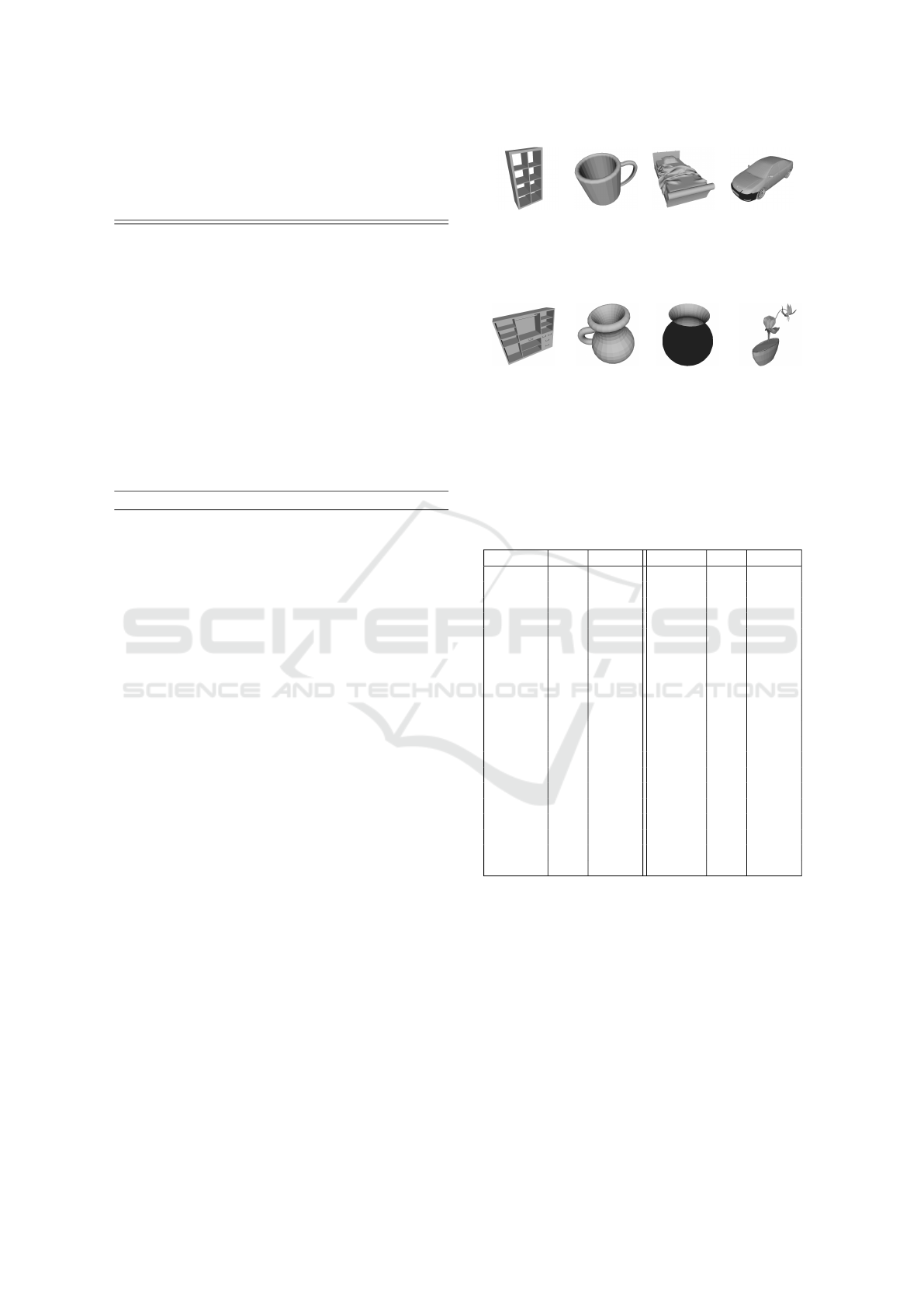
Table 4: Average accuracies on the ModelNet10 and Model-
Net40 datasests for some state-of-the-art methods from the
literature and for the proposed method.
Approach MN10 MN40
(Wu et al., 2015) 83.5% 77.0%
(Shi et al., 2015) 85.5% 77.6%
(Maturana and Scherer, 2015) 92.0% 83.0%
(Klokov and Lempitsky, 2017) 94.0% 91.8%
(Zanuttigh and Minto, 2017) 91.5% 87.8%
(Zhi et al., 2017) 93.4% 86.9%
(Xu and Todorovic, 2016) 88.0% 81.3%
(Johns et al., 2016) 92.8% 90.7%
(Wu et al., 2016) 91.0% 83.3%
(Brock et al., 2016) 97.1% 95.5%
(Sinha et al., 2016) 88.4% 83.9%
(Bai et al., 2016) 92.4% 83.1%
(Simonovsky and Komodakis, 2017) 90.0% 83.2%
(Hegde and Zadeh, 2016) 93.1% 90.8%
(Sfikas et al., 2017) 91.1% 90.7%
Proposed Method 93.6% 89.3%
shown in Table 5, while some examples of correctly
and wrongly classified objects are shown in Fig. 5 and
6 respectively. The accuracy is high on most classes
except for a few of them, e.g., the flower pot and radio
classes. These correspond to classes with a limited
amount of training samples and a large variability be-
tween the samples for which the algorithm is not able
to properly learn the structure. Inter-class similari-
ties are also more common given the larger number
of fine-grain classes present in the subset. In general,
classes sharing a similar appearance are more chal-
lenging to disambiguate, leading the model to confuse
e.g. table instances with desk instances. Similarly,
flower pot instances are often misclassified as plant
or vase while a number of cup instances have been
wrongly assigned to the vase category (some exam-
ples in these classes are shown in Fig. 6).
The comparison with competing approaches on
the ModelNet40 dataset is also reported in Table 4.
In this case our approach ranks 6th out of 15 com-
pared methods. Even if the relative ranking is slightly
lower than in the previous case this is still a very good
performance.
Finally concerning the training time, it is about 22
hours for the ModelNet10 dataset and 51 hours for the
larger ModelNet40 dataset (these are the numbers for
the complete version of the approach, using all the
three representations). The tests have been performed
on a system equipped with a 3.60 GHz Intel i7-4790
CPU and an NVIDIA TitanX (Pascal) GPU.
Bookshelf Cup Bed Car
574 94 518 203
Figure 5: Examples of 3D models from the ModelNet40
dataset correctly recognized by the proposed approach.
Wardrobe Cup Flower pot Flower pot
95 93 153 150
(Bookshelf ) (Vase) (Vase) (Plant)
Figure 6: Examples of 3D models from the ModelNet40
dataset wrongly recognized by the proposed approach. The
predicted categories are reported in parenthesis.
Table 5: Accuracy of the proposed approach on the various
classes of the ModelNet40 dataset. The number of samples
belonging to each class is also reported.
Class Acc. Samples Class Acc. Samples
airplane 100% 100 laptop 100% 20
bathtub 90% 50 mantel 94% 100
bed 97% 100 monitor 99% 100
bench 80% 20 night st. 76% 86
bookshelf 97% 100 person 100% 20
bottle 96% 100 piano 89% 100
bowl 100% 20 plant 91% 100
car 97% 100 radio 60% 20
chair 96% 100 r. hood 94% 100
cone 90% 20 sink 70% 20
cup 65% 20 sofa 96% 100
curtain 80% 20 stairs 75% 20
desk 84% 86 stool 90% 20
door 95% 20 table 77% 100
dresser 80% 86 tent 90% 20
flower pot 15% 20 toilet 97% 100
glass box 96% 100 tv st. 84% 100
guitar 93% 100 vase 74% 100
keyboard 100% 20 wardrobe 80% 20
lamp 75% 20 xbox 70% 20
6 CONCLUSIONS
In this paper we proposed a deep learning frame-
work for 3D objects classification. We used a multi-
branch architecture in which different representations
extracted from the object are exploited. Three dif-
ferent data representations have been evaluated. In
particular, maps containing the voxel densities proved
to be a compact yet very informative set of descrip-
tors. We also considered surface curvatures, an ap-
proach never exploited before, which proved to be a
Deep Learning for 3D Shape Classification based on Volumetric Density and Surface Approximation Clues
323

reliable solution with remarkable results. The pro-
posed approach requires a relatively small training ef-
fort, while it is able to achieve a state-of-the-art per-
formance on the ModelNet dataset. In the current ap-
proach, accuracies reported for volumetric and curva-
ture descriptors are slightly lower than those obtained
with depth data, future work will be devoted to im-
prove their performance as well. Furthermore, we
will explore the possibility of using more advanced
deep learning schemes and different approaches to
combine the multiple information sources.
REFERENCES
Bai, S., Bai, X., Zhou, Z., Zhang, Z., and Jan Latecki, L.
(2016). Gift: A real-time and scalable 3d shape search
engine. In Proceedings of CVPR, pages 5023–5032.
Brock, A., Lim, T., Ritchie, J. M., and Weston, N.
(2016). Generative and discriminative voxel modeling
with convolutional neural networks. arXiv preprint
arXiv:1608.04236.
Couprie, C., Farabet, C., Najman, L., and LeCun, Y. (2013).
Indoor semantic segmentation using depth informa-
tion. In Int. Conf. on Learning Representations.
Farabet, C., Couprie, C., Najman, L., and LeCun, Y.
(2013). Learning hierarchical features for scene la-
beling. IEEE Transactions on Pattern Analysis and
Machine Intelligence, 35(8):1915–1929.
Garcia-Garcia, A., Gomez-Donoso, F., Garcia-Rodriguez,
J., Orts-Escolano, S., Cazorla, M., and Azorin-Lopez,
J. (2016). Pointnet: A 3d convolutional neural net-
work for real-time object class recognition. In Pro-
ceedings of IJCNN, pages 1578–1584. IEEE.
Guo, Y., Bennamoun, M., Sohel, F., Lu, M., and Wan,
J. (2014). 3d object recognition in cluttered scenes
with local surface features: A survey. IEEE Trans-
actions on Pattern Analysis and Machine Intelligence,
36(11):2270–2287.
Hegde, V. and Zadeh, R. (2016). Fusionnet: 3d object clas-
sification using multiple data representations. arXiv
preprint arXiv:1607.05695.
Johns, E., Leutenegger, S., and Davison, A. J. (2016).
Pairwise decomposition of image sequences for ac-
tive multi-view recognition. In Proceedings of CVPR,
pages 3813–3822.
Klokov, R. and Lempitsky, V. (2017). Escape from cells:
Deep kd-networks for the recognition of 3d point
cloud models. arXiv preprint arXiv:1704.01222.
Li, B., Lu, Y., Li, C., Godil, A., Schreck, T., Aono, M.,
Burtscher, M., Chen, Q., Chowdhury, N. K., Fang,
B., et al. (2015). A comparison of 3d shape retrieval
methods based on a large-scale benchmark supporting
multimodal queries. Computer Vision and Image Un-
derstanding, 131:1–27.
Li, Y., Pirk, S., Su, H., Qi, C. R., and Guibas, L. J. (2016).
Fpnn: Field probing neural networks for 3d data. In
Advances in Neural Information Processing Systems.
Maturana, D. and Scherer, S. (2015). Voxnet: A 3d convolu-
tional neural network for real-time object recognition.
In International Conference on Intelligent Robots and
Systems (IROS), pages 922–928. IEEE.
Minto, L., Pagnutti, G., and Zanuttigh, P. (2016). Scene seg-
mentation driven by deep learning and surface fitting.
In Geometry Meets Deep Learning ECCV Workshop.
Pagnutti, G. and Zanuttigh, P. (2016). Joint color and depth
segmentation based on region merging and surface fit-
ting. In Proceedings of VISAPP.
Qi, C. R., Su, H., Mo, K., and Guibas, L. J. (2017). Pointnet:
Deep learning on point sets for 3d classification and
segmentation. In Proceedings of CVPR.
Qi, C. R., Su, H., Nießner, M., Dai, A., Yan, M., and
Guibas, L. J. (2016). Volumetric and multi-view cnns
for object classification on 3d data. In Proceedings of
CVPR, pages 5648–5656.
Sfikas, K., Theoharis, T., and Pratikakis, I. (2017). Ex-
ploiting the PANORAMA Representation for Convo-
lutional Neural Network Classification and Retrieval.
In Eurographics Workshop on 3D Object Retrieval.
Shi, B., Bai, S., Zhou, Z., and Bai, X. (2015). Deeppano:
Deep panoramic representation for 3-d shape recogni-
tion. IEEE Signal Processing Letters, 22(12):2339–
2343.
Simonovsky, M. and Komodakis, N. (2017). Dynamic
edge-conditioned filters in convolutional neural net-
works on graphs. In Proceedings of CVPR.
Sinha, A., Bai, J., and Ramani, K. (2016). Deep learning 3d
shape surfaces using geometry images. In Proceed-
ings of ECCV, pages 223–240. Springer.
Su, H., Maji, S., Kalogerakis, E., and Learned-Miller, E.
(2015). Multi-view convolutional neural networks for
3d shape recognition. In Proceedings of ICCV, pages
945–953.
Tangelder, J. W. and Veltkamp, R. C. (2004). A survey of
content based 3d shape retrieval methods. In Proceed-
ings of IEEE Int. Conference on Shape Modeling Ap-
plications, pages 145–156.
Theano Development Team (2016). Theano: A Python
framework for fast computation of mathematical ex-
pressions. arXiv e-prints, abs/1605.02688.
Wu, J., Zhang, C., Xue, T., Freeman, B., and Tenenbaum,
J. (2016). Learning a probabilistic latent space of ob-
ject shapes via 3d generative-adversarial modeling. In
Advances in Neural Information Processing Systems.
Wu, Z., Song, S., Khosla, A., Yu, F., Zhang, L., Tang, X.,
and Xiao, J. (2015). 3d shapenets: A deep representa-
tion for volumetric shapes. In Proceedings of CVPR,
pages 1912–1920.
Xu, X. and Todorovic, S. (2016). Beam search for learning
a deep convolutional neural network of 3d shapes. In
Proceedings of ICPR, pages 3506–3511. IEEE.
Zanuttigh, P. and Minto, L. (2017). Deep learning for 3d
shape classification from multiple depth maps. In Pro-
ceedings of ICIP.
Zhi, S., Liu, Y., Li, X., and Guo, Y. (2017). Lightnet: A
lightweight 3d convolutional neural network for real-
time 3d object recognition. In Eurographics Workshop
on 3D Object Retrieval.
VISAPP 2018 - International Conference on Computer Vision Theory and Applications
324
