
Tackling Demand Stochasticity by Redistribution among Retailers in a
Two-stage Distribution System
Benedikt De Vos and Birger Raa
Department of Industrial Systems Engineering and Product Design, Ghent University,
Technologiepark 903, 9000 Ghent, Belgium
Keywords:
Supply Chain Collaboration, Lateral Transshipments, Inventory Control, Inventory-routing.
Abstract:
This paper considers a two-stage distribution system consisting of a supplier supplying several retailers with
stochastic demand rates. Replenishments by the supplier happen cyclically, based on average retailer demand
rates. Hence, the considered distribution problem between the suppliers and its retailers is a Cyclic Inventory
Routing Problem (CIRP), which we solve with a state-of-the-art heuristic solution method. To cope with the
demand stochasticity, lateral transshipments can happen between retailers in each time period. We propose
a redistribution policy that determines the quantities being redistributed through lateral transshipments based
on the desired level of customer service the retailers want to reach (using the desired fill rate) and their actual
inventory levels. The cost of the daily redistribution is determined by solving a Travelling Salesman Problem
(TSP) covering the participating retailers. The potential benefits of the collaboration among retailers are
analyzed by comparing the distribution costs, the redistribution costs, the inventory holding costs and the
costs of lost sales at the retailers in different scenarios.
1 INTRODUCTION
Routing and inventory control often represent a large
part of a company’s operational costs. Traditionally,
operations management focused on optimizing the in-
ternal operations of a company. However, researchers
and companies realized that operational performance
does not only depend on their own decisions, but also
on the decisions made by other players in the sup-
ply chain. Hence, focus shifted from single-firm op-
timization to a more global ’supply chain manage-
ment’ perspective to create higher operational effi-
ciency. (Mentzer et al. (2001); Power (2005))
In this paper, a combination of vertical (i.e.,
among players on subsequent levels of the supply
chain) and horizontal (i.e., among players on the same
level of the supply chain) collaboration is introduced
in a distribution network. We consider a two-echelon
supply chain consisting of a supplier and his retailers.
Vertical collaboration between the supplier and his
retailers is established through Vendor-Managed In-
ventory (VMI). The retailers share demand data with
the supplier and hand over the responsibility for the
replenishment timing and quantity to the supplier.
This way, the supplier can coordinate retailer replen-
ishments better and design more efficient routes. The
supplier is then faced with an integrated inventory and
vehicle routing problem known as the Cyclic Inven-
tory Routing Problem (CIRP). VMI has been exten-
sively studied and comprehensive overviews of the
existing literature are given by Moin and Salhi (2007),
Andersson (2010) and Coelho (2013).
Horizontal collaboration is established among the
retailers through lateral transshipments, which en-
ables them to cope with demand uncertainty. Lat-
eral transshipments were defined by Tagaras (1999) as
”the redistribution of stock from retailers with stock
on hand to retailers that cannot meet customer de-
mands or retailers that expect significant losses due to
high risk”. Lateral transshipments can lead to service
improvement by preventing stockouts and to reduced
inventory holding costs. Previous research made a
distinction in redistribution based on the timing of the
lateral transshipments. Redistribution can take place
at predetermined times before all demand is realized
(i.e., proactive transshipments), or at any time to re-
spond to (potential) stockouts (i.e., reactive transship-
ments). Paterson (2011) gives a review on inventory
models with lateral transshipments.
A large part of the literature on lateral transship-
ments focuses solely on inventory control, assumes a
periodic inventory review policy, only considers one
232
Vos, B. and Raa, B.
Tackling Demand Stochasticity by Redistribution among Retailers in a Two-stage Distribution System.
DOI: 10.5220/0006623202320238
In Proceedings of the 7th International Conference on Operations Research and Enterprise Systems (ICORES 2018), pages 232-238
ISBN: 978-989-758-285-1
Copyright © 2018 by SCITEPRESS – Science and Technology Publications, Lda. All rights reserved

moment for redistribution within the order cycle or
lets lateral transshipments take place between only a
limited number of inventory points (Paterson et al.
(2011)). This paper contributes to this literature by
combining routing and inventory control at the retail-
ers through lateral transshipments. We develop an op-
erational model to determine the costs of redistribu-
tion and to analyze the benefits.
2 PROBLEM DESCRIPTION
We consider a two-echelon distribution network con-
sisting of a single supplier S who delivers a single
product to a retailer set I. The supplier cyclically re-
plenishes the retailers under a VMI system, based on
the retailers’ mean demand rates d
i
. The actual de-
mand rates at the retailers a
i,t
(i.e., the demand rate at
retailer i in time period t) are assumed to be stochastic
with a known probability distribution.
To cope with demand uncertainty, lateral trans-
shipments among the retailers are possible. The quan-
tities that are redistributed are determined by the re-
distribution policy. This policy is aimed at achiev-
ing a target service level at all retailers. Hence, the
redistributed quantities are based on the retailers’ in-
ventory levels and their fill rates. Since redistribution
will only involve relatively small quantities of goods
(compared to the supplier deliveries), we assume that
redistribution can be performed by a single vehicle.
We develop an operational solution method to de-
sign a cyclic distribution plan for the supplier to re-
plenish the retailers and a redistribution policy among
the retailers that realizes the potential benefits result-
ing from lateral transshipments. The solution method
determines the distribution cost, the cost of lateral
transshipments, the inventory holding cost at the re-
tailers and the cost of lost sales. These costs are com-
pared between the baseline system in which no lat-
eral transshipments occur and the collaborative sys-
tem with lateral transshipments. Given that redistri-
bution brings along additional costs, these have to be
balanced with the potential benefits of lower inven-
tory holding costs and lower lost sales.
3 DISTRIBUTION SOLUTION
ALGORITHM FOR THE CIRP
The distribution routes of the supplier are designed
using the two-phase route and fleet design CIRP
heuristic (Raa and Dullaert (2017)).
In the first phase of the CIRP heuristic, the
vehicle routes are designed using a construct-and-
improvement heuristic. An initial solution is con-
structed using a savings-based heuristic based on
the Clarke-and-Wright heuristic (Clarke and Wright
(1964)), which was adapted for the CIRP. The initial
solution is improved by using local search operators
(2-opt, relocate and exchange operators). Each local
search operator is reiterated until no more improve-
ment is found before moving on the the next operator.
A best-accept strategy is used per operator.
The route cycle times are chosen such that the dis-
tribution and inventory holding costs are minimized.
Every time a route r is made, it incurs a distribution
cost F
r
consisting of a vehicle loading and dispatch
cost, the delivery costs at the subset I
r
(i.e., the set
of retailers served by route r), and the transportation
costs to drive the route (i.e., the TSP tour visiting the
depot and the retailers in the route). To reduce dis-
tribution costs, the time between iterations of route r,
i.e. the cycle time T
r
, should be as long as possible.
Contrary to the distribution costs, the inventory
holding costs at the retailers that are covered by a
route increases with the route’s cycle time. The de-
livery quantity of retailer i is d
i
T
r
. Hence, the average
inventory level is
d
i
T
r
2
and the inventory holding cost
rate is
η
i
T
r
d
i
2
, with η
i
the holding cost per item per pe-
riod. The total cost rate TC
r
of route r thus varies with
the cycle time T
r
:
TC
r
=
F
r
T
r
+ T
r
∑
i∈I
r
η
i
d
i
2
(1)
The cycle time is however restricted by the vehi-
cle capacity κ and the storage capacity of the retailers
κ
i
, resulting in a maximum cycle time T
max,r
(cfr. for-
mula 2). The retailers in route r are visited each T
r
days, so they receive a delivery of d
i
T
r
items. This
delivery quantity should be lower than the storage ca-
pacity of the retailers κ
i
. Hence, the cycle time must
be less than or equal to min
i∈r
κ
i
d
i
. Further, when mak-
ing the route r, the vehicle is loaded with
∑
i∈r
d
i
T
r
items. This load should be lower than the vehicle ca-
pacity κ, so the cycle time T
r
cannot be higher than
κ
∑
i∈r
d
i
.
T
max,r
=
min
κ
∑
i∈r
d
i
, min
i∈r
κ
i
d
i
(2)
There is an optimal cycle time T
∗
r
that balances the
holding cost and the route cost and hence minimizes
the cost rate.
T
∗
r
= min
s
2F
r
∑
i∈r
η
i
d
i
!
, T
max,r
) (3)
Tackling Demand Stochasticity by Redistribution among Retailers in a Two-stage Distribution System
233

The total distribution cost rate equals the sum of
all the routes r ∈ R that the supplier has to perform to
replenish all his retailers I:
TC
S
=
∑
r∈R
TC
r
(4)
The first phase of the CIRP algorithm thus divides
the set of retailers into subsets that are each covered
by a separate route and for which the route cycle time
is chosen to minimize the cost rate.
The second phase of the CIRP algorithm assigns
the routes to vehicles and to specific periods using a
construct-and-improvement heuristic. The sequence
of the routes stays the same, but their cycle times can
be adjusted to minimize the required number of vehi-
cles and thus the fleet costs.
The construction heuristic is a best-fit insertion
heuristic that inserts the routes into the schedule in
such a way that the cumulative remaining time of the
vehicles to which the routes are assigned is minimal.
The routes are inserted in the schedule using two cy-
cle time selection rules. Firstly, the routes are inserted
with cycle times as close as possible to their optimal
cycle time (resulting in minimal route cost rates). Or
secondly, they are inserted with cycle times as close
as possible to their maximal cycle times (resulting in
minimal fleet cost rate). This results in two initial
schedules that are passed on to the improvement step.
In the improvement step, two local search operators
are applied, namely removing any single route from
the schedule and reinserting it in the cheapest possi-
ble spot, or removing all routes made by the vehicle
with the lowest utilization from the schedule en rein-
serting them in the cheapest possible way. To escape
a potential local optimum, the schedule that results
from the improvement step is scrambled by shuffling
route allocations. Local search is then repeated on the
scrambled solution. A predefined number of scram-
bles is set as a stopping criterion for the improvement
step.
The two-phase route and fleet design approach is
then reiterated within a metaheuristic framework (Raa
and Dullaert (2017)).
4 REDISTRIBUTION STRATEGY
AMONG RETAILERS
Once the routes and their allocation to vehicles are
known, the supplier can execute his distribution plan.
Then, the actual daily demand values a
i,t
are observed
for all retailers in each period. These demand rates
are generated using their known probability distribu-
tion. Since these demand values deviate from the av-
erage demand values, the actual inventory levels and
the resulting inventory holding costs will differ from
the inventory holding costs resulting from the CIRP
solution and have to be recalculated. Hence, in order
to know the actually incurred distribution cost rate,
the inventory holding costs (T
r
∑
i∈I
r
η
i
d
i
2
) have to be
subtracted from the routes’ cost rates TC
r
.
Further, inventory levels may be lower than antici-
pated (after periods with higher than average demand)
and the risk of stockout may occur. This is when re-
distribution through lateral shipments is activated.
Given that the cycle times of the routes can differ,
the time periods in which the retailers are replenished
will also differ from one retailer to another. Hence,
we allow redistribution in each time period across a
certain planning horizon.
At the start of period t, every retailer i has an in-
ventory level SI
i,t
. The ending inventory of retailer i
in that period EI
i,t
is calculated by subtracting the de-
mand in that period from the start inventory (= SI
i,t
-
a
i,t
). Redistribution is assumed to happen ’overnight’
between the periods, so the starting inventory level
of the next period also includes any lateral transship-
ments.
The redistribution quantities are thus determined
based on the ending inventory level of the retailers.
The retailers are divided into three different groups
in each time period. The retailers whose ending in-
ventory is too low to reach a certain desired service
level until their next delivery from the supplier, are
called receivers (1). Retailers whose ending inventory
is more than necessary to reach their desired service
level are called contributors (2). Finally, there are the
retailers that do not want to participate to the redis-
tribution in a specific period (3). The group to which
a retailer belongs can differ from one period to the
next, since his ending inventory will change accord-
ing to his incurred demand rate, redistributed quanti-
ties from the previous period and possible deliveries
from the supplier.
The desired service level is expressed by the fill
rate (i.e., the fraction of demand filled from items
available in inventory). For each time period, three
inventory levels are determined for each retailer, the
critical inventory level CI
i,t
, the threshold inventory
level TI
i,t
and the optimal inventory level OI
i,t
. The
critical inventory level CI
i,t
of a retailer is the inven-
tory level below which he wants to receive goods from
other retailers. So, a retailer is a receiver in time pe-
riod t if EI
i,t
<CI
i,t
. The threshold inventory level TI
i,t
is the inventory level above which he is willing to
share goods with other retailers. Hence, a retailer is
a contributor in time period t if EI
i,t
>TI
i,t
. The opti-
mal inventory level OI
i,t
of a retailer is the inventory
ICORES 2018 - 7th International Conference on Operations Research and Enterprise Systems
234

level up to which he wants to receive items from the
other retailers when his inventory has fallen below his
critical inventory level. If the inventory of retailer i in
time period t lies in the interval [CI
i,t
;TI
i,t
], he will not
participate in the redistribution in time period t. The
fill rates determining the critical inventory level and
the threshold inventory level of a retailer can change
over the time periods, depending on how many time
periods there are left before he receives his next order
from the supplier (i.e., the lead time L).
Based on the critical inventory level, the optimal
inventory level and the threshold inventory level of a
retailer, the number of goods he wants to contribute
(c
i,t
) or receive (r
i,t
) in a time period t can be deter-
mined.
c
i,t
= EI
i,t
− T I
i,t
(5)
r
i,t
= OI
i,t
− EI
i,t
(6)
When the contributor amount (
∑
i
c
i,t
) equals the
receiver amount (
∑
i
r
i,t
), they can be optimally redis-
tributed. However, these amounts will often be dif-
ferent. When the contributor amount is smaller than
the receiver amount (
∑
i
c
i,t
<
∑
i
r
i,t
), the receivers will
not all be able to reach their optimal inventory level,
so an appropriate decision rule is required to divide
the contributed items over the receivers. Conversely,
when
∑
i
c
i,t
>
∑
i
r
i,t
, we need to decide what contribu-
tors will contribute which quantities.
These decisions are also taken based on the fill
rates of the receivers and the contributors. When
the contributors want to contribute more items than
receivers want to receive (
∑
i
c
i,t
>
∑
i
r
i,t
), the con-
tributed items are collected from the contributors in
such a way that they end up with a new inventory
level that results in the same fill rate for the contribu-
tors (which is still above the required fill rate). When
the receivers want to receive more items than the con-
tributors want to contribute, the contributed items are
allocated over the receivers in such a way they all end
up with a new inventory level with the same fill rate
(which is still below the required fill rate). The num-
ber of items a retailer i actually receives or contributes
in period t are denoted as R
i,t
and C
i,t
.
When the received and contributed number of
items for all retailers are calculated at the end of time
period t, the start inventory level of the retailers in the
next period SI
i,t+1
can be calculated. This is done by
adding the quantity delivered by the supplier in that
time period D
i,t+1
(which will be zero when no deliv-
ery occurs in that time period), subtracting the number
of contributed items C
i,t
and adding the number of re-
ceived items R
i,t
from the end inventory level EI
i,t
in
period t. The end inventory level EI
i,t
in all time peri-
ods is determined by subtracting the incurred demand
a
i,t
from the start inventory level SI
i,t
. Note that this
end inventory level can become negative. When it is
negative, it means that retailer i could not meet the de-
mand and lost sales occur (LS
i,t
). In periods in which
the end inventory of a retailer is higher than or equal
to zero, no lost sales occur (i.e. LS
i,t
= 0). When the
end inventory is lower than zero, lost sales amount to
-EI
i,t
. Note that the formula for the start inventory SI
i,t
takes into account lost sales from the previous period.
D
i,t
=
(
0 if there is no delivery in t
d
i
T
r
if there is a delivery in t
(7)
SI
i,t
= max(0, EI
i,t−1
) + D
i,t
+ R
i,t−1
−C
i,t−1
(8)
EI
i,t
= SI
i,t
− a
i,t
(9)
LS
i,t
= −min(0, EI
i,t
) (10)
Besides the cost of distribution and redistribution,
the cost of lost sales and the inventory holding cost at
the retailers are also considered to assess the collab-
orative supply chain with lateral transshipments. The
lost sales cost rate of a retailer LSC
i
is calculated by
taking his average number of lost sales per time pe-
riod and multiplying it with the cost of one item that
could not be sold (λ
i
) (cfr. formula 11). To calculate
the inventory holding cost rate of a retailer H
i
, his av-
erage inventory in each time period is summed over
the planning horizon and multiplied with his inven-
tory holding cost per item per time period (η
i
) divided
by the number of time periods in the planning horizon
p (cfr. formula 12).
LSC
i
=
λ
i
P
∑
t∈P
LS
i,t
(11)
H
i
=
η
i
P
∑
t∈P
SI
i,t
+ EI
i,t
2
(12)
Note that this new inventory holding cost at the re-
tailers replaces the inventory holding cost calculated
in the CIRP solution algorithm (T
r
∑
i∈I
r
η
i
d
i
2
, cfr. for-
mula 1), since it is the inventory holding cost that the
retailers will actually incur.
To determine the daily redistribution cost, a TSP
is solved each day. The nodes in the TSP on a spe-
cific day are the receivers and the contributors. We
assume there is no limitation on the capacity of the
third party courier, since the redistributed volumes
are small. The model takes into account a travel cost
per km (θ). The redistribution cost rate is calculated
Tackling Demand Stochasticity by Redistribution among Retailers in a Two-stage Distribution System
235
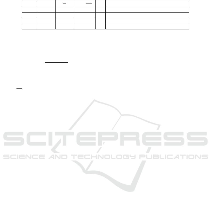
Table 1: CIRP routes supplier illustrative example.
r TC
r
F
r
T
r
∑
i∈r
η
i
d
i
2
T
r
Sequence
1 139 64 75 4 S → 8 → 4 → 5 → 2 → S
2 172.66 99.16 73.5 5 S → 10 → 1 → 11 → 7 → 13 → 12 → S
3 224 149.3 74.7 3 S → 6 → 14 → 3 → 15 → 9 → S
Total 535.66 312.46 223.2
by multiplying the distances resulting from the TSPs
with the travel cost per km and taking the average over
the planning horizon P.
RC =
∑
t∈P
T SP
t
.θ
P
(13)
The total cost comprises the distribution cost rate
of the supplier TC
s
(minus the inventory holding
cost at the retailers incorporated in this cost rate
(
∑
i∈I
r
T
r
η
i
d
i
2
)), the redistribution cost rate RC, the
sum of the inventory holding cost over all retailers
(
∑
i∈I
H
i
) and the sum of the lost sales cost over all
retailers (
∑
i∈I
LSPC
i
). This total cost is computed
for the baseline system without lateral transshipments
and for the cooperative system with lateral transship-
ments. Both cases are compared to identify the bene-
fits of the lateral transshipments.
5 ILLUSTRATIVE EXAMPLE
The suggested solution approach is illustrated with an
illustrative example. The example comprises one sup-
plier replenishing 15 retailers with one type of prod-
uct. One time period is assumed to be one day. The
average daily demand rates of the retailers d
i
are gen-
erated randomly between 0.2 and 10 items per day
and their maximum storage capacity between 10 and
100 items. The inventory holding cost and the lost
sales cost of the retailers are assumed to be equal
for all retailers and are respectively 1.5/item/day and
100/item. The retailers’ locations are generated ran-
domly in such a way that they are uniformly dis-
tributed in a circle around the supplier
The routes resulting from the CIRP algorithm are
shown in Table 1. The total transportation cost rate
of the supplier TC
S
equals 535.66 (= 139 + 172.66 +
224). The inventory holding costs of the retailers have
to be subtracted from the routes’ cost rates. These
inventory holding cost rates amount to 75, 73.5 and
74.7. So, the transportation cost rates that are taken
into account for the comparison of the baseline sys-
tem without lateral transshipments and the collabora-
tive system with lateral transshipments are 64 (= 139
- 75), 99.16 (=172.66 - 73.5) and 149.3 (= 224 - 74.7),
summing to a total transportation cost rate of 312.46.
The daily demand rates of the retailers are as-
sumed to be normally distributed with mean d
i
and
standard deviation 0.1 d
i
. Given that the cycle times
of the routes of the suppliers are 4, 5 and 3, actual
daily demand rates are generated for all retailers over
a planning horizon of 60 days (= P). Table 2 shows the
actual daily demand rates for retailer 2 over 12 days.
These demand rates are generated based on his aver-
age demand rate of 4.6 and standard deviation 0.46.
The supplier receives a delivery of 18.4 items (= 4 .
4.6) on days 1, 5 and 9 since the cycle time of his
route is 4. Based on the actual demand rates, the start
and end inventory levels of the retailers in the base-
line system without lateral transshipments can be cal-
culated using formulas 8 and 9. The negative end in-
ventory levels on days 4, 8 and 12 (resp. -0.3, -0.9 and
-1.0 items) indicate that a stockout (and consequently
lost sales) occurs on these days due to the higher than
average demand over the previous days. Note that the
lost sales cannot be backlogged, so the start inventory
on day 5 equals the delivery retailer 2 receives from
the supplier and does not take into account the lost
sales of 0.3 from day 4.
The cost of lost sales and the inventory holding
cost are calculated for all retailers (cfr. formulas 11
and 12). Table 3 shows the overall lost sales cost rate
and inventory holding cost rate in the baseline system
without lateral transshipments over all retailers. The
total cost rate in the baseline system without redistri-
bution equals 618.11 (= 312.46 + 254.15 + 51.5).
When redistribution is introduced, the threshold
inventory level, the optimal inventory level and the
critical inventory level are calculated for all retailers
on all days. In our example, we assume a fill rate of
99.5% for the threshold inventory level, 99% for the
optimal inventory level and 98.5% for the critical in-
ventory level. Table 4 shows the three inventory levels
for retailer 2 over 12 days. Note that on day 1 the in-
ventory levels are calculated using a lead time of 3
since it is the inventory level at the end of the day that
is compared to the threshold inventory level, the opti-
mal inventory level and the critical inventory level. At
the end of day 1, retailer 2 expects his next delivery in
3 days. Hence, the lead time of 3 days.
Based on these inventory levels and the end inven-
tory level of the retailers, the receiver and contributor
ICORES 2018 - 7th International Conference on Operations Research and Enterprise Systems
236
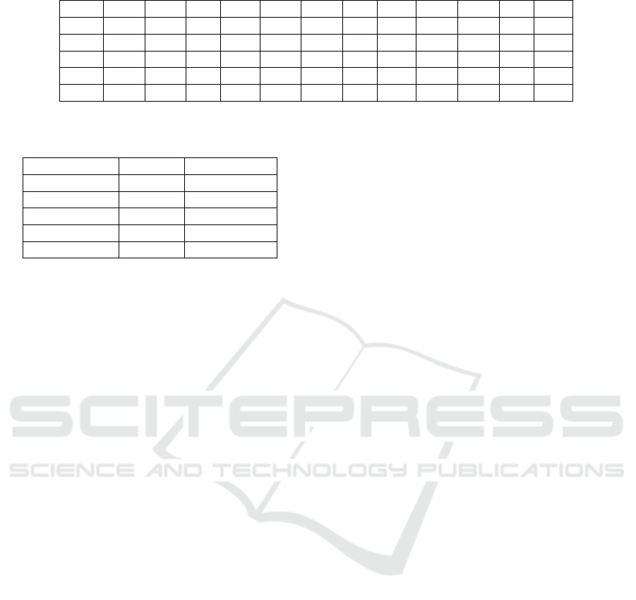
Table 2: Retailer 2 days 1 to 12 illustrative example baseline system.
t 1 2 3 4 5 6 7 8 9 10 11 12
D
2,t
18.4 0 0 0 18.4 0 0 0 18.4 0 0 0
a
2,t
4.3 4.2 4.9 5.3 5.4 4.6 5 4.3 4.9 4.9 4.4 5.2
SI
2,t
18.4 14.1 9.9 5.0 18.4 13.0 8.4 3.4 18.4 13.5 8.6 4.2
EI
2,t
14.1 9.9 5.0 -0.3 13.0 8.4 3.4 -0.9 13.5 8.6 4.2 -1.0
LS
2,t
0 0 0 0.3 0 0 0 0.9 0 0 0 1
Table 3: Lost sales, inventory holding, distribution and re-
distribution cost rates.
Baseline Collaborative
∑
i
LSC
i
51.50 23.50
∑
i
H
i
254.15 244.00
TC
S
312.46 312.46
RC 0.00 31.84
Total cost rate 618.11 611.80
amounts are determined. On day 2 for example, the
end inventory of retailer 2 is higher than his threshold
inventory (9.9>9.7), so he is willing to hand over 0.2
items to the other retailers. Table 4 also shows the to-
tal receiver and contributor amount (resp.
∑
i
r
i,t
and
∑
i
c
i,t
) over all retailers over the 12 days. On day 2
there are more receiver items requested than there are
items contributed (1.2<3.1). Hence, supplier 2 will
contribute the total 0.2 items. The receiver and con-
tributor quantities are redistributed ’overnight’. So,
the start inventory of retailer 2 on day 3 is updated for
these 0.2 contributed items (9.9 - 0.2 = 9.7). On day
5 on the other hand, the end inventory of retailer 2
falls below his critical inventory (13.2<13.9). So, re-
tailer 2 is a receiver on that day. The total contributor
amount is now higher than the total receiver amount
(4.4>0.8), so retailer 2 will receive his full number
of requested items (0.7). Again, the start inventory of
retailer 2 on day 6 takes into account this number of
received items (13.2 + 0.7 = 13.9).
The new lost sales of retailer 2 in the 12-day pe-
riod are also included in table 4. These are determined
in the same way as in the baseline system (i.e., as the
negative end inventory when the end inventory falls
below zero). Note that despite the redistribution of in-
ventory among the retailers, retailer 2 incurs lost sales
on day 4. Overall, his lost sales are lower than in the
baseline sytem though (0.3 + 0.9 + 1).
The number of lost sales, the average inventory
level and the corresponding lost sales cost rate and in-
ventory holding cost rate is calculated over all retail-
ers in the planning horizon in the collaborative sys-
tem with lateral transshipments. The results are also
shown in Table 3. The lost sales cost rate has dropped
(-54.3%) compared to the baseline system, as has the
inventory holding cost rate (-3.9%). However, the
cost of redistribution has to be taken into account. A
TSP is solved for each day within the 60-days plan-
ning horizon. On day 7 for example, retailers 2 and 13
want to receive items (resp. 0.1 and 0.9 items). They
receive these items from retailers 4, 9 and 10. So, on
day 7 a TSP is solved among retailers 2, 4, 9, 10 and
13. The total redistribution cost rate resulting from
the TSPs over the planning horizon equals 31.84.
The collaborative system with lateral transship-
ments among the retailers results in our example
only in a small decrease in the total cost rate (-
1,02%). However, lost sales have decreased consider-
ably (from 30.9 items to 14.1 items over the 60-days
planning horizon), so the customer service level has
improved too.
6 CONCLUSIONS
We studied the benefits of lateral transshipments of in-
ventory among retailers in a two-stage supply chain.
The supplier replenishes the retailers in a VMI setting
and his/her distribution routes and distribution cost
are determined using a CIRP solution heuristic. Re-
plenishments by the supplier are periodic. However,
since the replenishment frequencies are determined in
the CIRP heuristic, cycle times of the retailers can
differ from one to another. Redistribution of inven-
tory is possible in all time periods. The redistributed
quantities are determined based on the inventory level
of the retailers and their desired fill rate. The bene-
fits of the lateral transshipments are savings created
through reductions in lost sales and inventory hold-
ing costs and increased customers service levels. The
cost reductions have to be balanced with the increase
in transportation cost caused by the redistribution of
inventory. The cost of redistribution is determined by
solving TSP problems among the retailers that want
to participate in the redistribution.
Preliminary results show that savings in inventory
costs and lost sales can occur through lateral trans-
shipments in the VMI setting. Furthermore, the cus-
tomer service levels increase. However, the savings
are highly dependent on the problem parameters, like
the cost of lost sales, the inventory holding cost at the
Tackling Demand Stochasticity by Redistribution among Retailers in a Two-stage Distribution System
237
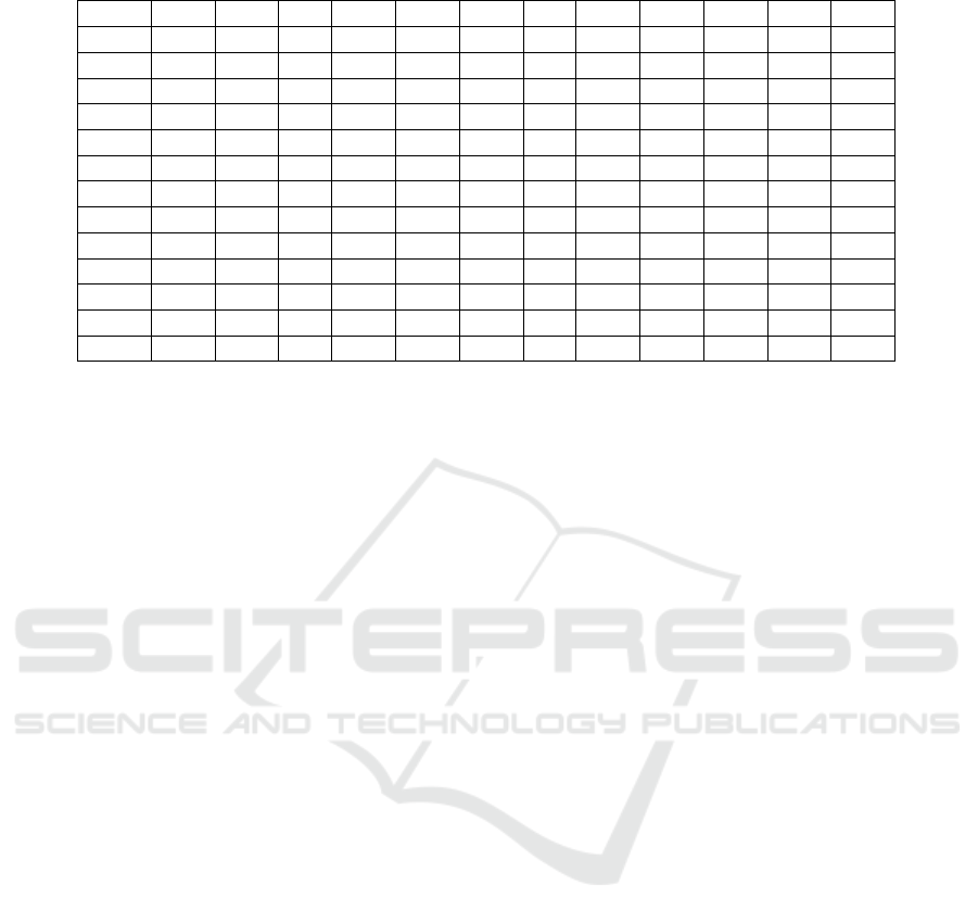
Table 4: Retailer 2 days 1 to 12 illustrative example collaborative system.
t 1 2 3 4 5 6 7 8 9 10 11 12
D
2,t
18.4 0 0 0 18.4 0 0 0 18.4 0 0 0
L 3 2 1 4 3 2 1 4 3 2 1 4
T I
2,t
14.5 9.7 4.8 19.2 14.5 9.7 4.8 19.2 14.5 9.7 4.8 19.2
OI
2,t
14.1 9.4 4.6 18.9 14.1 9.4 4.6 18.9 14.1 9.4 4.6 18.9
CI
2,t
13.9 9.2 4.4 18.6 13.9 9.2 4.4 18.6 13.9 9.2 4.4 18.6
a
2,t
4.3 4.2 4.9 4.3 5.4 4.6 5 4.3 4.9 4.9 4.4 5.2
SI
2,t
18.4 14.1 9.7 4.8 18.6 13.9 9.3 4.4 18.6 13.9 9.2 4.8
EI
2,t
14.1 9.9 4.8 -0.5 13.2 9.3 4.3 0.1 13.7 9 4.8 -0.4
C
2,t
0 0.2 0 0 0 0 0 0 0 0 0 0
R
2,t
0 0 0 0.2 0.7 0 0.1 0.1 0.2 0.2 0 0.2
∑
i
c
i,t
0.1 1.2 0.6 4.7 4.4 3.1 7.2 7.1 9.5 10.6 11.3 10.5
∑
i
r
i,t
3.3 3.1 2.3 0.6 0.8 1.5 1 0.2 0.5 0.2 0.5 0.7
LS
2,t
0 0 0 0.5 0 0 0 0 0 0 0 0.4
retailers and the location of the retailers (and conse-
quently the cost of distribution and redistribution).
More in-depth research into larger datasets is nec-
essary. A design of experiments should be performed
to calibrate the redistribution policy parameters across
a wide range of instances. The chosen levels of the
fill rate to determine the threshold, critical and op-
timal inventory levels appear to have a large impact
on the quantities all retailers want to contribute or re-
ceive to the redistribution, and consequently on the
redistribution costs. Also the way in which we deter-
mine which retailers actually contribute items when
the contributor amount is higher than the receiver
amount (or vice versa, when the amount of receiver
items is higher than the contributor amount) must be
investigated more in detail. The preliminary analy-
sis showed for example that it can be beneficial to
exclude some retailers from the redistribution in cer-
tain time periods to prevent unnecessary movements
of small quantities and to keep the redistribution cost
resulting from the TSP under control. These redistri-
bution policy parameters become certainly important
in more realistic datasets with a high number of retail-
ers.
Furthermore, when determining which retailers
should contribute and receive what quantities in the
redistribution, we must keep in mind that all retailers
want to receive benefits when entering the collabora-
tion. Hence, the benefits should be shared over all
participants in a fair way, otherwise some participants
will be inclined to leave the collaboration. Further
research can be performed on how all retailers can re-
ceive a fair share of the redistribution benefits.
Additionally, taking into account demand variabil-
ity into the CIRP to reduce the need for redistribution
should also be investigated.
ACKNOWLEDGEMENTS
This research was supported by the Agency for In-
novation by Science and Technology in Flanders
(VLAIO).
REFERENCES
Andersson, H. et al. (2010). Industrial aspects and literature
survey: Combined inventory management and rout-
ing. Computers & Operations Research, 37(9):1515–
1536.
Clarke, G. and Wright, J. W. (1964). Scheduling of vehicles
from a central depot to a number of delivery points.
Operations Research, 12(4):568–581.
Coelho, L. C. et al. (2013). Thirty years of inventory rout-
ing. Transportation Science, 48(1):1–19.
Mentzer, J. T. et al. (2001). Defining supply chain manage-
ment. Journal of Business Logistics, 22(2):1–25.
Moin, N. and Salhi, S. (2007). Inventory routing problems:
a logistical overview. Journal of the Operational Re-
search Society, 58(9):1185–1194.
Paterson, C. et al. (2011). Inventory models with lateral
transshipments: A review. European Journal of Oper-
ational Research, 210(2):125–136.
Power, D. (2005). Supply chain management integration
and implementation: a literature review. Supply chain
management: an international journal, 10(4):252–
263.
Raa, B. and Dullaert, W. (2017). Route and fleet design for
cyclic inventory routing. European Journal of Opera-
tional Research, 256(2):404–411.
Tagaras, G. (1999). Pooling in multi-location periodic in-
ventory distribution systems. Omega, 27(1):39–59.
ICORES 2018 - 7th International Conference on Operations Research and Enterprise Systems
238
