Combining 2D to 2D and 3D to 2D Point Correspondences for Stereo
Visual Odometry
Stephan Manthe
1
, Adrian Carrio
2
, Frank Neuhaus
1
, Pascual Campoy
2
and Dietrich Paulus
1
1
Institute for Computational Visualistics, University of Koblenz-Landau, Universit
¨
atsstr. 1, 56070 Koblenz, Germany
2
Computer Vision & Aerial Robotics Group, Universidad Polit
´
ecnica de Madrid,
Calle Jos
´
e Guti
´
errez de Abascal, 28006 Madrid, Spain
Keywords:
Visual Stereo Odometry, Epipolar Constraint, Bundle Adjustment.
Abstract:
Self-localization and motion estimation are requisite skills for autonomous robots. They enable the robot to
navigate autonomously without relying on external positioning systems. The autonomous navigation can be
achieved by making use of a stereo camera on board the robot. In this work a stereo visual odometry algorithm
is developed which uses FAST features in combination with the Rotated-BRIEF descriptor and an approach for
feature tracking. For motion estimation we utilize 3D to 2D point correspondences as well as 2D to 2D point
correspondences. First we estimate an initial relative pose by decomposing the essential matrix. After that
we refine the initial motion estimate by solving an optimization problem that minimizes the reprojection error
as well as a cost function based on the epipolar constraint. The second cost function enables us to take also
advantage of useful information from 2D to 2D point correspondences. Finally, we evaluate the implemented
algorithm on the well known KITTI and EuRoC datasets.
1 INTRODUCTION
Stereo visual odometry (VO) is a method to compute
the egomotion of a camera system relative to a sta-
tic scene that consists of two cameras. Stereo VO al-
gorithms continuously compute the relative poses be-
tween two consecutive points in time from overlap-
ping images captured by the camera system. By con-
catenating these relative poses they continuously up-
date an absolute pose that describes the camera pose
with relation to an arbitrary initial pose. In order to
estimate the motion over time, VO algorithms track
image parts and make use of structure from motion
techniques to derive the camera system’s motion and
3D structure of the captured scene.
Recently, many applications of VO have been
found in the field of robotics, since motion estimation
is essential for many robotic tasks. One reason for
the high interest of VO in robotics are the advantages
of the sensor properties. Due to their wide applica-
tions also in consumer devices: they are cheap, with
a small form factor and lightweight. However, this
comes with the cost of the need to process images,
which is computationally expensive and can be error
prone in scenarios with bad lighting conditions.
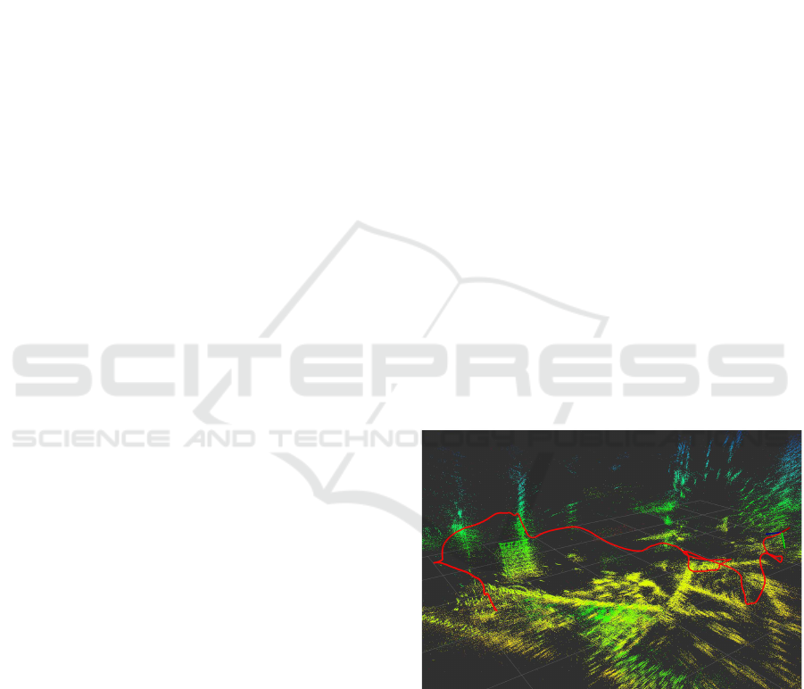
Figure 1: Reconstructed trajectory and point cloud. The
trajectory is visualized in red and the point cloud is colored
based on elevation. On the right of the image the current
position of the camera marked by a coordinate system can
be seen.
In this work we adapt the depth enhanced odome-
try approach of Zhang et al. to a pure stereo vision
based approach (Zhang et al., 2014). This enables
us to exploit the previously described advantages of a
pure camera based sensor system. In contrast to their
approach we triangulate features using stereo image
Manthe, S., Carrio, A., Neuhaus, F., Campoy, P. and Paulus, D.
Combining 2D to 2D and 3D to 2D Point Correspondences for Stereo Visual Odometry.
DOI: 10.5220/0006623604550463
In Proceedings of the 13th International Joint Conference on Computer Vision, Imaging and Computer Graphics Theory and Applications (VISIGRAPP 2018) - Volume 5: VISAPP, pages
455-463
ISBN: 978-989-758-290-5
Copyright © 2018 by SCITEPRESS – Science and Technology Publications, Lda. All rights reserved
455

pairs instead of associating 2D features with depth
information from a depth map. Following their ap-
proach, we utilize features with and without depth to
maximize information gain. However, we propose for
this a slightly modified version of their cost function
for features without depth information which returns
a metric error and is essentially based on the epipo-
lar constraint (Hartley and Sturm, 1997). This ena-
bles our algorithm to be extended by tightly coupled
sensor fusion since it allows a normalization of the
error terms. In contrast to the algorithm of Zhang
et al. we do not implement windowed bundle adjus-
tment (BA) and focus on pure frame to frame motion
estimation, which can be considered a pairwise BA
algorithm. This keeps processing times low and ena-
bles us to apply our algorithm on board a robot with
low computational power which is an unmanned ae-
rial vehicle in our case. BA is a further step that im-
proves the results of the very first step related to cal-
culating VO from two consecutive stereo image pairs.
This is the reason why we focus our work in this pa-
per on this first step, that can of course be improved
by a further BA upon the improvements we present in
this paper. We evaluate the proposed algorithm exten-
sively on two different datasets and present evaluation
results that are similar to that of Zhang et al.
The rest of this paper is structured as follows. In
Section 2 we present the related work. After that, we
revise in Section 3 important basic knowledge before
we give an overview of our algorithm in Section 4. In
Section 5 we introduce our algorithm more in detail
followed by the evaluation of our approach on two
different datasets in Section 6. Finally our work is
summarized in Section 7.
2 RELATED WORK
A lot of work on VO has been done by the Robo-
tics and Perception group at ETH Z
¨
urich, led by Da-
vide Scaramuzza. His two-part tutorial gives an over-
view to common algorithms used in VO (Scaramuzza
and Fraundorfer, 2011; Fraundorfer and Scaramuzza,
2012). In these tutorials also visual-SLAM techni-
ques which are related to VO are explained.
Cvi
ˇ
si
´
c and Petrovi
´
c recently achieve very accu-
rate results with their method on the KITTI odome-
try benchmark (Cvi
ˇ
si
´
c and Petrovi
´
c, 2015). They
focus on careful feature selection by making use of
two different keypoint detection algorithms. This al-
lows them to have a high feature acceptance thres-
hold while keeping still enough features for motion
estimation. In contrast to our work the motion esti-
mation of their algorithm is divided into rotation esti-
mation and translation estimation separately. First the
rotation matrix is extracted from an estimated essen-
tial matrix and then the translation vector is estimated
by iteratively minimizing the reprojection error with
a fixed rotation matrix.
Buczko et al. also focused on outlier rejection in
order to achieve high accuracy during motion estima-
tion. The authors presented a new iterative outlier
rejection scheme (Buczko and Willert, 2016b) and
a new flow-decoupled normalized reprojection error
(Buczko and Willert, 2016a). Their method achieves
as well outstanding results in translation and rotation
accuracy on the KITTI odometry benchmark.
The work in this paper is based on the idea of com-
bining information of image features with and wit-
hout known depth information developed by Zhang
et al. They build an odometry system that combines
a monocular camera with a depth sensor. Their al-
gorithm assigns to the tracked features in the camera
images depth information from the depth sensor if this
information is available. During their motion estima-
tion they utilize features with and without depth in
order to achieve a maximum information gain when
recovering the motion. The use of features without
depth enables to compute a relatively accurate pose
even if only a few features with depth information
are available. They evaluated their method with an
Asus Xtion Pro Live RGB-D camera and a sensor sy-
stem consisting of a camera in combination with a
Hokuyo UTM-30LX laser scanner on their own da-
tasets. Additionally they also evaluated on the public
KITTI dataset which provides the depth information
from a Velodyne HDL-64E laser scanner. Our method
differs from theirs as it obtains metric depth informa-
tion from a stereo camera and it does not use BA. As
mentioned before, we also apply a small adaption of
their cost function for 2D to 2D point corresponden-
ces.
Fu et al. compute the depth information of
Zhang’s algorithm by using a stereo camera also (Fu
et al., 2015). However, they do this by using a
block matching algorithm. Furthermore their algo-
rithm uses key frames which can reduce the drift in
situations where the camera is not moving. Also the
rest of their motion estimation is similar to Zhang’s
approach since they apply their motion estimation ap-
proach including BA for their camera system.
3 THEORETICAL BACKGROUND
The VO approach described in this paper solves a BA
problem in order to estimate the most likely motion
given two stereo image pairs from consecutive points
VISAPP 2018 - International Conference on Computer Vision Theory and Applications
456
in time. For this, an optimization problem is setup
that makes use of the epipolar geometry, which des-
cribes the geometrical properties between two came-
ras. Furthermore, the epipolar geometry will also be
used during the feature matching process in our algo-
rithm. In this section, the basics of epipolar geometry
will be described in order to give a better insight into
our algorithm.
The relative pose between two cameras is des-
cribed as a rigid transformation given by a rota-
tion matrix R ∈ IR
3×3
and a translation vector t =
(t
x
, t
y
, t
z
)
T
∈ IR
3
. These can be used to transform an
arbitrary 3D point that is defined in the coordinate sy-
stem of a camera c
1
into the coordinate system of a
second camera c
2
. With R and t we can also define
the so called essential matrix
E = R[t]
×
, (1)
where [t]
×
is a skew symmetric matrix
[t]
×
=
0 −t
z
t
y
t
z
0 −t
x
−t
y
t
x
0
. (2)
It maps a homogeneous undistorted point ˜p
i
in image
coordinates of the first camera to a homogeneous
line
˜
l in image coordinates of the second camera
˜
l = E ˜p
i
. (3)
The projections of any point located on a ray inter-
secting the projection center of the first camera and
p
i
are projected onto this line. Given the homoge-
neous undistorted point ˜q
i
in image coordinates of the
second camera, we compute the corresponding homo-
geneous line
˜m = E
T
˜q
i
(4)
where ˜m is in image coordinates of the first camera.
The constraint that a corresponding point in the se-
cond image of a point from the first image has to lie
on an epipolar line is named the epipolar constraint.
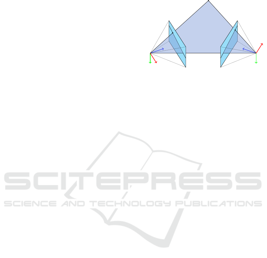
This geometric relation is depicted in Figure 2 and
will be used during motion estimation as well as fea-
ture matching.
Another approach to compute the essential ma-
trix is to use point correspondences from two ima-
ges. This can be done for example by using the 5-
point-algorithm which computes the essential matrix
from 5 point correspondences (Nist
´
er, 2004). Since
often many more correspondences are available and
not all of them are correct it is often used in combina-
tion with a RANSAC framework. It robustifies the al-
gorithm and classifies the point correspondences into
inliers and outliers. The computed essential matrix
can then be decomposed into a rotation matrix R and
c
1
c
2
˜m
˜
l
˜p
i
˜q
i
Figure 2: Illustration of the epipolar geometry and the epi-
polar constraint.
a translation vector t. As a result, two possible rota-
tions R and R
T
as well as two possible translations t
and −t are obtained. Thus the four possible solutions
have to be validated by checking the cheirality con-
straint. It describes that a 3D point lies in front of both
cameras from which it was reconstructed. Therefore,
it is determined with which of the four possible solu-
tions the largest number of 3D points can be correctly
triangulated. Finally the relative pose from which the
most correct triangulated 3D points can be obtained
is chosen (Hartley, 1993). The interested reader may
find a more detailed description of how to extract the
correct R and t from an essential matrix in (Hartley
and Zisserman, 2003). However, by making use of 2D
to 2D point correspondences t can only be estimated
up to a scale factor. The scale factor can be recovered
from known 3D to 2D point correspondences as we
show in Section 5.
4 ALGORITHM OVERVIEW
The stereo VO algorithm presented in this work uses
a feature-based approach. It extracts FAST features
(Rosten et al., 2010) from images and guarantees an
equal distribution of them by means of bucketing in
the left and right stereo image (Zhang et al., 1995).
The oriented-BRIEF descriptor is then applied to
the filtered keypoints (Rublee et al., 2011). Even
though FAST is an undirected keypoint extraction
algorithm and oriented-BRIEF cannot make use of
its rotational invariance, we achieved more precise
motion estimation results with it. These probably
come from the machine learning stage of the modi-
fied BRIEF descriptor. At the end of the feature ex-
traction stage we transform all keypoints into undis-
torted image coordinates in order to avoid repeated
distortion and undistortion during the following pro-
cessing.
In order to match keypoints between the left and
the right stereo camera we utilized stereo matching al-
Combining 2D to 2D and 3D to 2D Point Correspondences for Stereo Visual Odometry
457

ong epipolar lines only. This allows to exclude many
wrong matches, which are not possible due to the epi-
polar constraint. We apply the stereo matching twice
from the left to the right image and vice versa. Only
if the matching results in the same correspondence in
both cases, it will be accepted as a correct match.
The search for keypoint correspondences over
time is only done in the left image. For this purpose
we applied the KLT-tracker on the extracted FAST
keypoints (Lucas and Kanade, 1981). During our tests
the tracking of keypoints lead to many more keypoint
correspondences than a keypoint matching approach
and has also been applied in other works (Zhang et al.,
2014; Cvi
ˇ
si
´
c and Petrovi
´
c, 2015).
For point cloud triangulation between the
keypoints in the left and the right image we used the
optimal triangulation method presented by Hartley
and Sturm (Hartley and Sturm, 1997). By using
these 3D points, the algorithm derives 3D to 2D
point correspondences between time t − 1 and t by
concatenating the results of the previously described
matching and tracking phases. Since our algorithm
is a pure VO algorithm it maintains the keypoint
correspondences only while they are needed for the
following motion estimation. For the purpose of
visualization the algorithm keeps the triangulated 3D
points in memory without any further processing.
In the next phase, the algorithm estimates the re-
lative motion as a rigid transformation between two
successive points in time. This phase is split up into
a motion initialization and a motion refinement step
which are described in more detail in Section 5. Af-
ter the relative pose is computed, it is concatenated
with the initial absolute pose. In the second iteration
and every following iteration the relative pose is con-
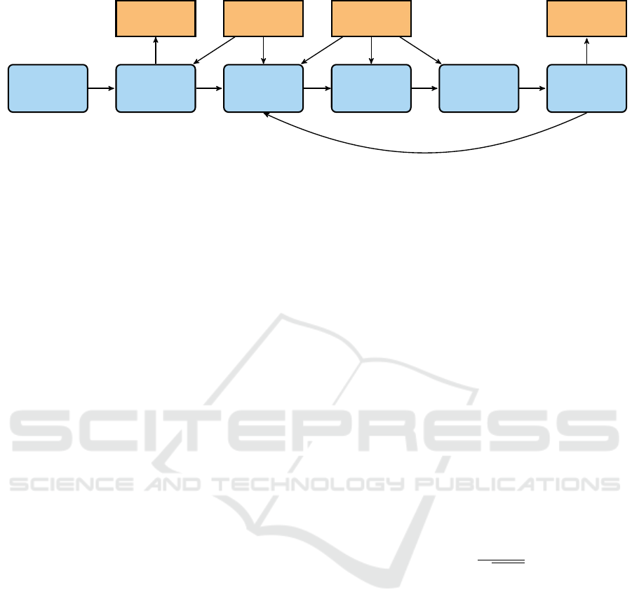
catenated with the previous absolute pose. Figure 3
shows a diagram that visualizes the whole pipeline of
our algorithm.
5 MOTION ESTIMATION
Our motion estimation algorithm estimates for a pe-
riod of time ∆t between two points in time t and t − 1
the motion of the left camera as a rigid transforma-
tion. It is a pure frame to frame motion estimation
and split up into two consecutive steps. The first step
is an initial motion estimation that estimates the es-
sential matrix first and then extracts the relative pose
from it. With this pose, BA respectively a nonlinear
optimization problem is initialized in a second step. It
minimizes both the reprojection error and an error that
measures how good the current estimated pose fulfills
the epipolar constraint.
5.1 Motion Initialization
Our motion initialization needs 2D to 2D keypoint
correspondences as well as 3D to 2D keypoint cor-
respondences as an input. All 2D to 2D correspon-
dences that are available from the matching will be
used for estimating an essential matrix between two
camera poses of the left camera from different points
in time. After that the scale of the translation is deri-
ved from 3D to 2D point correspondences.
Step 1: Essential Matrix Computation. For mo-
tion initialization, first the essential matrix E
∆t
is es-
timated. This is done using a 5-point-algorithm that is
embedded into a RANSAC framework (Nist
´
er, 2004).
All point correspondences which were classified as
outliers by the RANSAC algorithm are not used du-
ring the computation of the motion initialization. This
makes the computation robust against wrong keypoint
matches as well as moving keypoints which result
from moving objects.
Step 2: Extraction of the Relative Pose. From E
∆t
the relative pose of the stereo camera between the two
points in time is computed. It is defined by the rota-
tion matrix R
∆t
and the translation vector t
0
∆t
that is
defined up to a scale factor. Both are computed from
E
∆t
by the method described in Section 3. For the ini-
tial pose R
∆t
can be used directly but the correct scale
of t
0
∆t
has to be estimated first since it can have large
errors.
Step 3: Scale Computation of the Translation.
The scale of t
0
∆t
can be computed from a 3D point
p
c
=
p
c
x
, p
c
y
, p
c
z
T
, which was triangulated with the
correct scale from the stereo camera and a 3D point
p
0
=
p
0
x
, p
0
y
, p
0
z
T
with incorrect scale. The point p
0
was triangulated from a 2D to 2D point correspon-
dence of the left camera over time. For this R
∆t
and
t
0
∆t
with incorrect scale were used. In the next step the
scale factor α of p
0
is computed as:
α =
1
3
·
p
c
x
p
0
x
+
p
c
y
p
0
y
+
p
c
z
p
0
z
!
. (5)
It can be used to scale t
0
∆t
to its correct length. Ho-
wever, for being robust against outliers the scale is
computed for all point correspondences. From them
heuristically the 5% of the smallest and 5% of the lar-
gest scale factors are discarded, since they likely con-
tain outliers. With the n remaining scale factors, the
correct scaled translation vector is computed as
t
∆t
=
1
n
n
∑
k=0
α
k
· t
0
∆t
(6)
where α
k
is the k-th scale factor.
The method to derive the initial pose here pre-
sented is inspired by the method described in (Scara-
muzza and Fraundorfer, 2011) to derive a consistent
VISAPP 2018 - International Conference on Computer Vision Theory and Applications
458
Initialization
Store First
Image
Matching
and Tracking
Initial Pose
Stereo
Image Pairs
Point Cloud
Recon-
struction
Motion
Estimation
Replace
Stored Image
Computed
Pose
Sensor Unit
Calibration
Figure 3: Pipeline of the stereo VO algorithm. The figure depicts the single algorithmic steps and data flows during the
execution of the stereo VO algorithm. Therefore blue boxes with rounded corners indicate algorithmic processes and orange
boxes with sharp corners data. The arrows indicate the data flow.
scaled motion of a monocular camera from 2D to 2D
point correspondences. This method uses also trian-
gulated 3D points but without a metric and another
formula to estimate scale. Also the method for de-
riving the translation vector in (Cvi
ˇ
si
´
c and Petrovi
´
c,
2015) is similar in the way that it uses reconstructed
3D points triangulated with a metric scale from a pre-
vious stereo image pair. Here during an optimization
procedure the full translation vector whose scale is
derived from the triangulated 3D points is estimated.
However, the method presented here is to the best of
our knowledge not presented in the literature and the-
refore assumed to be new.
5.2 Motion Refinement
The goal of the motion refinement is to refine the co-
arse estimation of R
∆t
and t
∆t
from the motion initia-
lization. We achieve this by setting up a BA problem
that makes use of information from 2D to 2D as well
as 3D to 2D point correspondences. The first type of
cost function computes the well known reprojection
error which makes use of 2D to 3D point correspon-
dences. It is important since it is used to derive the
correct scale of the translation vector. In contrast the
second type of cost function uses 2D to 2D point cor-
respondences and quantifies how good two correspon-
ding points satisfy the epipolar constraint. The later
influences only the rotation matrix and the orientation
of the translation vector.
Reprojection Error. The reprojection error quanti-
fies the distance between a predicted projection of a
3D point and its corresponding observation for a gi-
ven pose of a camera. In order to compute the costs, a
3D point p
c
t−1
from time t −1 is transformed first into
the camera coordinate system of the camera at time t
p
c
t
= R
∆t
· p
c
t−1
+ t
∆t
. (7)
This one is then projected into image coordinates
p
i
t
= π (p
c
t
) (8)
where π is the projection function which computes the
projection of p
c
t
as a point p
i
t
in image coordinates.
Finally the reprojection error is defined as
r = kq
i
t
− p
i
t
k
2
(9)
where q
i
is the corresponding point to p
i
and k · k
2
is
the L
2
-norm.
Epipolar Error. The epipolar error used here quan-
tifies how good the epipolar constraint is satisfied for
a given relative pose and two corresponding 2D fea-
tures. This is done by measuring the metric distance
between a point and the epipolar line on which this
point should lie on. First from a homogeneous point
˜p
i
t−1
in image coordinates the epipolar line
˜
l
t
= E
∆t
· ˜p
i
t−1
(10)
is computed. In a next step the metric distance be-
tween the point ˜q
i
t
and
˜
l
t
=
˜
l
x
,
˜
l
y
,
˜
l
z
T
is computed.
Therefore we normalize
˜
l
t
as
¯
l
t
=
˜
l
t
·
1
q
˜
l
x
+
˜
l
y
(11)
and denote the normalized epipolar line with
¯
l
t
. After
that the distance between
˜
l
t
and ˜q
i
t
is computed as
e =
¯
l
t
T
· ˜q
i
t
. (12)
For the second point ˜q
i
t
of the point correspondence
the same error measure is computed again but by ma-
king use of E
T
∆t
.
These computations are similar to the ones done
by Zhang et al. since it can be shown that the cost
function for 2D to 2D point correspondences he pro-
posed also measures how good the current relative
pose fulfills the epipolar constraint. However, the cost
function he proposed does not work with normalized
lines and points. We decided to compute a metric dis-
tance since it allows us to define a heuristically es-
timated standard deviation. This is necessary for a
correct weighting between the two different kinds of
Combining 2D to 2D and 3D to 2D Point Correspondences for Stereo Visual Odometry
459

cost functions and it is also a preparation of our algo-
rithm for sensor fusion with inertial information for
example.
Like Zhang et al. we also weight our cost terms
with the Tukey biweight loss function (Huber, 2011).
It assigns a fixed value to costs that are higher than
a certain threshold. Since the result value of this
function does not change as long as the cost term is
higher than this threshold, these functions do not in-
fluence the optimization result. This is similar to an
outlier rejection of wrong keypoint correspondences.
However, since the costs of keypoint corresponden-
ces change during optimization it is possible that a
keypoint that produces costs over that threshold can
have influence on the optimization result again after
several iterations.
6 EVALUATION
For evaluating our algorithm we used a consumer
Laptop with an Intel
R
Core
TM
i7-4850HQ 2.30 GHz
CPU and 24 Gb RAM. We implemented the algorithm
in modern C++11 based on the robot operating system
(ROS) which we used for visualization as well as for
evaluation. For nonlinear optimization of the BA we
utilized the Ceres-Solver which ran in parallel with 8
threads (Agarwal et al., 2017). As evaluation datasets
we used the odometry dataset of the KITTI Vision
Benchmark Suite
1
(Geiger et al., 2012) and the Eu-
ropean Robotics Challenge
2
(EuRoC) dataset (Burri
et al., 2016).
For evaluation on the KITTI dataset we used the
rotation error e
rot
and translation error e
trans
which
are also used for evaluation by the KITTI odometry
benchmark suite (Geiger et al., 2012). It should give
an idea of about how good our algorithm performs
in comparison to the one by Zhang et al. Additio-
nally, we provide results for the absolute trajectory
error (ATE) (Sturm et al., 2012) which aims to mea-
sure the global consistency of a computed trajectory.
Its computation needs only information about the po-
sition of the camera system and not the orientation.
This is useful since for some EuRoC datasets only po-
sition information is provided.
6.1 Results on the KITTI Dataset
The odometry dataset of the KITTI Vision Bench-
mark Suite were recorded by a moving car. The 22
1
Web page of the KITTI Vision Benchmark Suite:
http://www.cvlibs.net/datasets/kitti/eval odometry.php
2
Web page of the EuRoC dataset: http://projects.asl.
ethz.ch/datasets/doku.php?id=kmavvisualinertialdatasets
Table 1: Evaluation results on KITTI dataset.
Dataset ATE [m] e
trans
[%] e
rot
[deg/m]
00 5.20 1.00 0.0032
01 - - -
02 8.57 0.94 0.0031
03 0.70 2.10 0.0034
04 3.11 2.96 0.0032
05 9.12 2.60 0.0054
06 8.12 2.73 0.0072
07 5.14 2.27 0.0104
08 11.29 2.35 0.0043
09 12.18 3.17 0.0046
10 4.99 2.05 0.0047
Average 6.84 2.22 0.0050
datasets are split into eleven training datasets and ele-
ven evaluation datasets. We evaluate our algorithm
only on the eleven training datasets since for the eva-
luation datasets no ground truth is public available.
The ground truth information of the datasets is provi-
ded as a 6D pose and computed from a GPS receiver
with an integrated IMU. The stereo camera system of
the car provides grayscale images at a frame rate of
10 frames per second and a resolution of 1241 × 376
pixels (Geiger et al., 2012).
During our experiments the algorithm matched
approximately 380 keypoints between the left and the
right image and tracked 1290 keypoints between two
consecutive images including outliers. As described
in Section 5.1 and Section 5.2 these outliers were pro-
perly handled by the RANSAC algorithm during mo-
tion initialization and the robust cost functions during
the motion refinement.
Our evaluation results are shown in Table 1. The
algorithm achieves the best results on the datasets 00
and 02 with relation to e
rot
and e
trans
. Except for da-
taset 01 our algorithm is able to compute the whole
trajectory for all datasets. During the processing of
dataset 01 the algorithm is not able to keep track of
the trajectory since the scale computation fails due to
the lack of proper feature correspondences. When the
scale computation fails many feature matches are lo-
cated far away on the horizon where the triangulated
depth information of 3D points can contain large er-
rors.
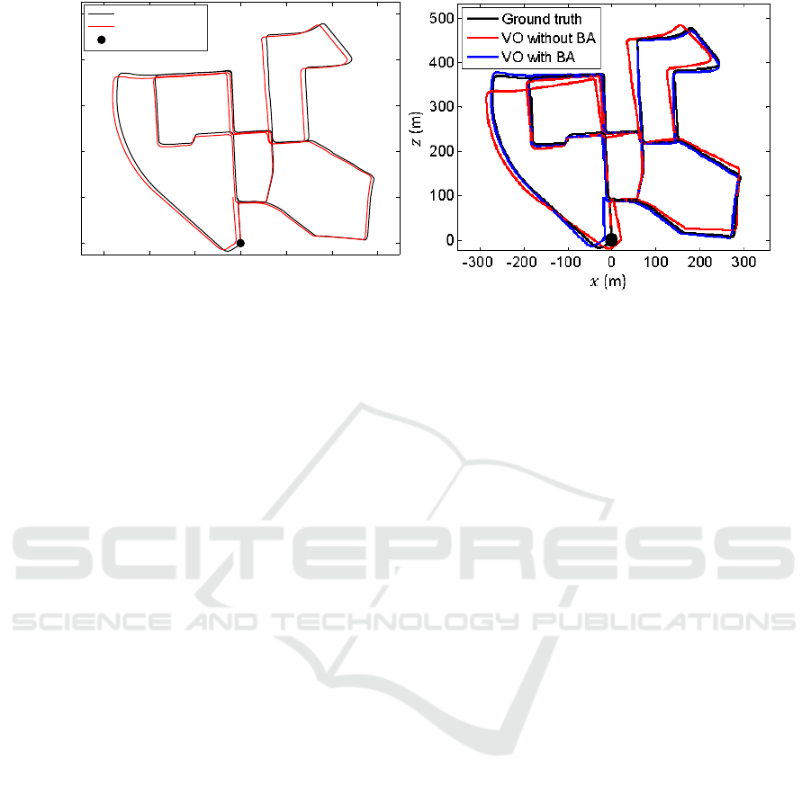
Figure 4(b) shows the trajectory of Zhang’s algo-
rithm in the ground plane with and without windowed
BA for the KITTI dataset 00. By comparing the tra-
jectory without windowed BA to the one with it, it can
be seen how much positive impact it has on the accu-
racy of the trajectories. Due to this fact, the results
of our algorithm cannot be compared with the results
of Zhang et al. since the authors of that work do not
provide evaluation data without windowed BA. Ho-
VISAPP 2018 - International Conference on Computer Vision Theory and Applications
460
−300 −200 −100 0 100 200 300
x (m)
0
100
200
300
400
500
y (m)
Ground Truth
Our Result
Start point
(a) KITTI 00 in the ground plane. (b) KITTI 00 in the ground plane by Zhang et al. (Zhang
et al., 2014).
Figure 4: Reconstructed trajectories in the ground plane for the dataset KITTI 00.
wever, in comparison to our trajectory visualized in
Figure 4(a) the trajectory of Zhang’s algorithm dif-
fers more from the ground truth trajectory than ours
in the ground plane.
The results of the ATE do not always correlate
with the translational error e
trans
. This apparent lack
of correlation can be attributed to the different charac-
teristics of the error measurements. Especially for tra-
jectories where the vehicle moves only straight ahead
like 03, 04, 07 and 10 this error is very low. In these
cases the computed and the ground truth trajectory
can be aligned very well, which happens during the
computation of the ATE.
The average error values in Table 1 were compu-
ted without considering dataset 01. The processing of
a single stereo image pair of the KITTI dataset took
approximately 180 milliseconds.
6.2 Results on the EuRoC Dataset
The EuRoC dataset contains data records captured
with a hexacopter (Burri et al., 2016). The robot was
equipped with a sensor system that provided synchro-
nized grayscale stereo image pairs which were cap-
tured with a resolution of 768 × 480 pixel at 20 Hz.
The datasets were captured in three different environ-
ments. The “Vicon Room 1” (V1) datasets are captu-
red in a bright room whereas “Vicon Room 2” (V2)
datasets were captured in the same room with less
light and different obstacles. From both environments
respectively datasets with three levels of difficulty:
V1-1 and V2-1 easy; V1-2 and V2-2 medium; V1-3
and V2-3 difficult. The different degrees of difficulty
result from different motion speeds and lighting con-
ditions. As ground truth a full 6D pose is provided.
The remaining 5 datasets were recorded in a “Ma-
chine Hall” (MH) environment. The degrees of dif-
ficulty are here also divided into three levels: MH-1
and MH-2 easy; MH-3 medium; MH-4 and MH-5 dif-
ficult. For these datasets only the ground truth posi-
tion is provided.
Since the resolution of the images from the Eu-
RoC dataset is smaller than for the KITTI dataset less
keypoint matches can be extracted from the images.
These were approximately 380 keypoints between the
left and the right image and 830 for consecutive ima-
ges.
Our evaluation results on the EuRoC dataset are
shown in Table 2. By examining the values of the ATE
it can be noticed that they are smaller than the ones
from the KITTI dataset in general. This comes from
the expansion of the trajectories which is in general
smaller than for the KITTI dataset. By further analy-
sis it can also be noticed that the algorithm seems to
perform better on the Machine Hall datasets. This is
the result of a slower optical flow in the image stream
since almost all objects are further away from the ca-
mera than in the Vicon Room datasets. The keypoint
matching and tracking profits from this. However, at
some parts of the trajectories for MH-4 and MH-5 the
algorithm is almost not able to track the camera sys-
tems egomotion due to bad lighting conditions. These
problems lead to high ATE values.
On the Vicon Room datasets the algorithm works
for the datasets with easy and medium degree of dif-
ficulty. For these datasets the algorithm is able to
handle the speed of the optical flow and the resulting
motion blur. Only for the datasets V1-3 and V2-3
our algorithm is not able to track the egomotion of
the camera. In these situations fast changing lighting
conditions which result in almost black images due
to the cameras auto exposure as well as strong mo-
Combining 2D to 2D and 3D to 2D Point Correspondences for Stereo Visual Odometry
461
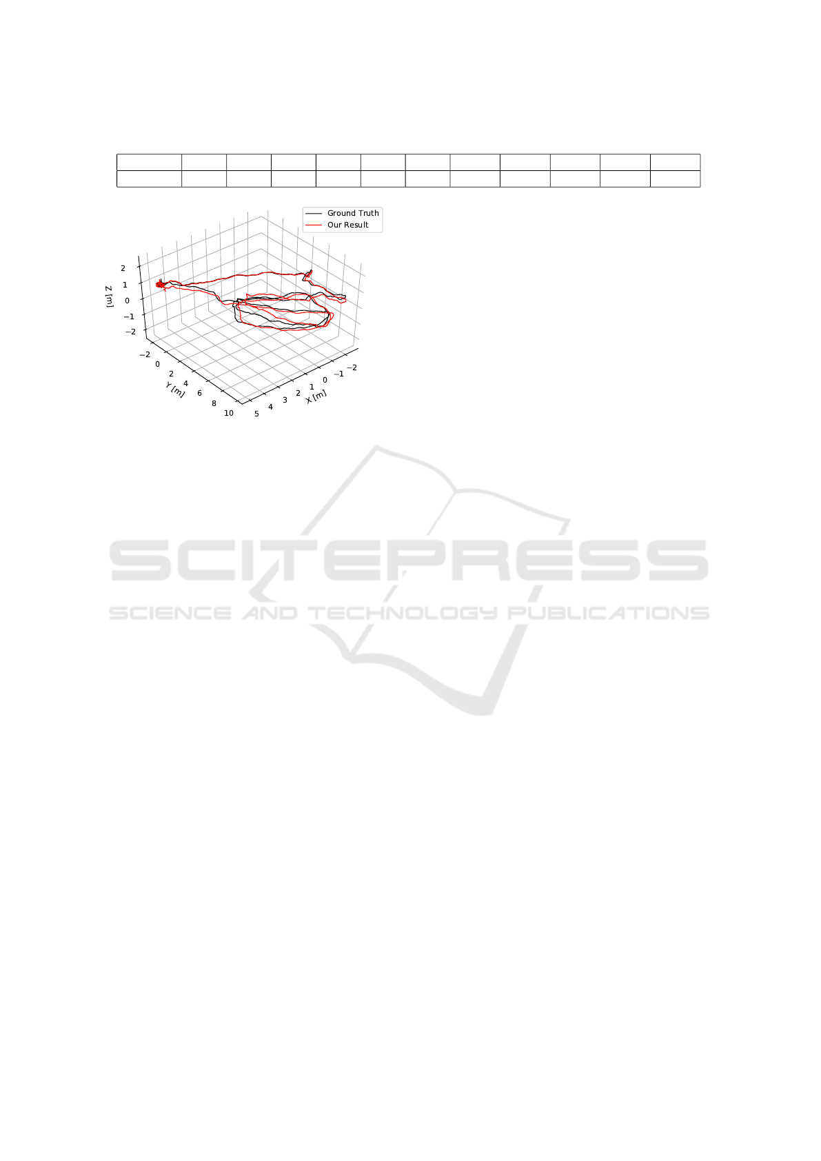
Table 2: Evaluation results on the EuRoC dataset.
Dataset V1-1 V1-2 V1-3 V2-1 V2-2 V2-3 MH-1 MH-2 MH-3 MH-4 MH-5
ATE [m] 0.60 0.35 - 0.51 0.85 - 0.19 0.21 0.63 1.64 1.52
Figure 5: Visualization of the trajectory of the dataset MH-2
in 3D. The trajectory was aligned by computing an optimal
transformation for the first 1100 positions. It can be noticed
that the trajectory starts to drift after a few meters. However,
the trajectory proceeds close to the ground truth even at its
end.
tion blur lead to few and wrong point corresponden-
ces. In consequence the relative pose estimation di-
verges at several points of the trajectory. In order to
overcome the problems resulting from motion blur, a
keypoint tracking method that applies the photometric
error could be utilized.
The processing time for a stereo image pair from
the EuRoC dataset took approximately 140 millise-
conds. This smaller processing time in comparison to
the KITTI dataset comes obviously from the smaller
image size of the dataset and fewer computed featu-
res.
7 CONCLUSION AND FUTURE
WORK
In this work we have presented a pure visual odome-
try approach which adapts the idea of Zhang et al.
(Zhang et al., 2014) to utilize keypoints with and wit-
hout known depth information during motion estima-
tion. In contrast to Zhang et al. we have used a stereo
camera instead of a laser scanner in order to obtain
depth information. Instead our algorithm computes
depth information from keypoint matches which are
obtained by means of keypoint matching and tracking.
These matches are passed to the motion estimation
which is split into a initialization and refinement step.
With our motion initialization we have shown how an
initial estimate for a nonlinear optimization problem
can be derived which is solved during motion refine-
ment. This optimization problem utilizes the infor-
mation from 2D to 2D as well as 3D to 2D keypoint
matches. With this approach we achieved promising
results on the well known EuRoC and KITTI dataset.
However, the algorithm was not able track the trajec-
tory in three cases where many triangulated keypoint
features were far away on the horizon or no keypoints
could be matched due to bad light conditions.
During further developments we would like to ex-
tend our approach with windowed BA which has the
potential to improve the accuracy of the trajectory
a lot. Additionally we also plan to utilize keypoint
correspondences from the right stereo camera in our
motion refinement. This may also make it possible
to avoid the motion initialization step and could also
enable the algorithm to keep track in environments
with bad lighting conditions.
ACKNOWLEDGEMENTS
We thank the German Academic Exchange Service
(DAAD) for partially founding this work.
REFERENCES
Agarwal, S., Mierle, K., and Others (2017). Ceres solver.
http://ceres-solver.org. Version 1.12.
Buczko, M. and Willert, V. (2016a). Flow-decoupled nor-
malized reprojection error for visual odometry. In In-
telligent Transportation Systems (ITSC), 2016 IEEE
19th International Conference on, pages 1161–1167.
IEEE.
Buczko, M. and Willert, V. (2016b). How to distinguish in-
liers from outliers in visual odometry for high-speed
automotive applications. In 2016 IEEE Intelligent
Vehicles Symposium (IV), pages 478–483. IEEE.
Burri, M., Nikolic, J., Gohl, P., Schneider, T., Rehder, J.,
Omari, S., Achtelik, M. W., and Siegwart, R. (2016).
The EuRoC micro aerial vehicle datasets. The Inter-
national Journal of Robotics Research.
Cvi
ˇ
si
´
c, I. and Petrovi
´
c, I. (2015). Stereo odometry based on
careful feature selection and tracking. In Mobile Ro-
bots (ECMR), 2015 European Conference on, pages
1–6. IEEE.
Fraundorfer, F. and Scaramuzza, D. (2012). Visual odome-
try: Part ii: Matching, robustness, optimization, and
applications. IEEE Robotics & Automation Magazine,
19(2):78–90.
VISAPP 2018 - International Conference on Computer Vision Theory and Applications
462

Fu, C., Carrio, A., and Campoy, P. (2015). Efficient visual
odometry and mapping for unmanned aerial vehicle
using arm-based stereo vision pre-processing system.
In Unmanned Aircraft Systems (ICUAS), 2015 Inter-
national Conference on, pages 957–962. IEEE.
Geiger, A., Lenz, P., and Urtasun, R. (2012). Are we ready
for autonomous driving? the KITTI vision benchmark
suite. In Proceedings of the IEEE Computer Society
Conference on Computer Vision and Pattern Recogni-
tion, pages 3354–3361.
Hartley, R. and Zisserman, A. (2003). Multiple view geome-
try in computer vision. Cambridge university press.
Hartley, R. I. (1993). Cheirality invariants. In Proc. DARPA
Image Understanding Workshop, pages 745–753.
Hartley, R. I. and Sturm, P. (1997). Triangulation. Computer
vision and image understanding, 68(2):146–157.
Huber, P. J. (2011). Robust statistics. In International En-
cyclopedia of Statistical Science, pages 1248–1251.
Springer.
Lucas, B. D. and Kanade, T. (1981). An iterative image re-
gistration technique with an application to stereo vi-
sion. In Proceedings of the 7th International Joint
Conference on Artificial Intelligence, IJCAI ’81, Van-
couver, BC, Canada, August 24-28, 1981, pages 674–
679.
Nist
´
er, D. (2004). An efficient solution to the five-point
relative pose problem. IEEE transactions on pattern
analysis and machine intelligence, 26(6):756–770.
Rosten, E., Porter, R., and Drummond, T. (2010). Faster
and better: A machine learning approach to corner
detection. IEEE transactions on pattern analysis and
machine intelligence, 32(1):105–119.
Rublee, E., Rabaud, V., Konolige, K., and Bradski, G.
(2011). Orb: An efficient alternative to sift or surf.
In Computer Vision (ICCV), 2011 IEEE International
Conference on, pages 2564–2571. IEEE.
Scaramuzza, D. and Fraundorfer, F. (2011). Visual odome-
try : Part I: The first 30 years and fundamentals. IEEE
Robotics & Automation Magazine, 18(4):80–92.
Sturm, J., Engelhard, N., Endres, F., Burgard, W., and Cre-
mers, D. (2012). A benchmark for the evaluation of
rgb-d slam systems. In 2012 IEEE/RSJ International
Conference on Intelligent Robots and Systems, pages
573–580. IEEE.
Zhang, J., Kaess, M., and Singh, S. (2014). Real-time depth
enhanced monocular odometry. In Intelligent Robots
and Systems (IROS 2014), 2014 IEEE/RSJ Internatio-
nal Conference on, pages 4973–4980. IEEE.
Zhang, Z., Deriche, R., Faugeras, O., and Luong, Q.-T.
(1995). A robust technique for matching two unca-
librated images through the recovery of the unknown
epipolar geometry. Artificial intelligence, 78(1-2):87–
119.
Combining 2D to 2D and 3D to 2D Point Correspondences for Stereo Visual Odometry
463
