
Data Mining Applied to Transportation Mode Classification Problem
Andrea Vassilev
CEA, LETI, MINATEC Campus F-38054, Grenoble, France
Keywords: Context Awareness, Transportation Mode, Data Mining, Classification, Smartphone, Sensors, Principal
Component Analysis, Mahalanobis Distance, Linear Discriminant Analysis.
Abstract: The recent increase in processing power and in the number of sensors present in today’s mobile devices leads
to a renewed interest in context-aware applications. This paper focuses on a particular type of context, the
transportation mode used by a person or freight, and adequate methods for automatically classifying
transportation mode from smartphone embedded sensors. This classification problem is generally solved by
a searching process which, given a set of design choices relative to sensors, feature selection, classifier family
and hyper parameters, etc., find an optimal classifier. This process can be very time consuming, due to the
number of design choices, the number of training phases needed for a cross validation step and the time
necessary for one training phase. In this paper, we propose to simplify this problem by applying three data
mining tools - Principal Component Analysis, Mahalanobis distance and Linear Discriminant Analysis - in
order to clean the data, simplify the problem and finally speed up the searching process. We illustrate the
different tools on the transportation mode classification problem.
1 INTRODUCTION
The field of context recognition has gathered a lot of
attention in recent years mostly thanks to the
widespread of mobile devices (for e.g. smartphones
and wearable). With the continuous integration of
new sensors, their ever increasing computing power
and their virtual omnipresence, these devices have
become ideal tools for context recognition. More
precisely, our interest here is the recognition of the
transportation modes used by a person or freight. The
applications are numerous:
Carbon footprint evaluation (Manzoni et al.,
2010),
Real-time door-to-door journey smart
planning,
Smart mobility survey (Nitsche et al., 2014),
Driving analysis (Vlahogianni and
Barmpounakis, 2017),
Road user analysis and collision prevention,
Goods mobility tracking
Traffic Management
This classification problem is generally solved by
a searching process which, given a set of design
choices find an optimal classifier.
A design choice involves 3 main aspects:
Sensors: modern mobile devices contain
several different sensors, at least the
following eight: accelerometer (ACC),
magnetometer (MAG), gyroscope,
barometer, GPS, Wifi, GSM, audio… Each
of these sensor can be used for transportation
mode classification. Most widely used are
ACC and GPS (Wu et al., 2016), (Stenneth
et al., 2011), (Hemminki et al., 2013),
(Reddy et al., 2010), but some authors use
only GSM (Anderson and Muller, 2006) or
only barometer (Sankaran et al., 2014). The
number of different sensor combinations
(for 8 sensors) is already important
(2
8
=256).
Features: raw sensor data are rarely used
directly, but are often pre-processed leading
to features. E.g., given the accelerometer
readings over a finite time window (E.g. 5
seconds.) on can compute the mean value,
the variance, the skewness, the number of
zero crossings, the Fast Fourier Transform
(FFT) coefficients, the energy for different
frequency bands,…
Given a set of sensors there is almost an
infinite number of features that can be
computed.
36
Vassilev, A.
Data Mining Applied to Transportation Mode Classification Problem.
DOI: 10.5220/0006633300360046
In Proceedings of the 4th International Conference on Vehicle Technology and Intelligent Transport Systems (VEHITS 2018), pages 36-46
ISBN: 978-989-758-293-6
Copyright
c
2019 by SCITEPRESS – Science and Technology Publications, Lda. All rights reserved

Classifier family and associated hyper
parameters: each classifier family (decision
tree (DT), neural network (NN),…) has its
own hyper parameters that need to be fixed
before training: e.g., for DT, the maximum
number of splits, for NN, the number of
hidden layers and the number of neurons by
layer,…
Testing different combinations of sensors, fea-
tures, classifiers and hyper-parameters often lead to a
rapid increase of the total number of design choices
N
D
(phenomenon known as combinatorial explosion).
Moreover, given a design choice, once a classifier
is trained, its classification performance has to be
evaluated. The most widely used technique is a
K-fold cross validation approach (Arlot and Celisse,
2010) which needs K+1 training phases, leading to a
total number ~N
D
.K of training phases.
Finally, the training phase duration is very
sensitive to the problem dimension, i.e. the number of
features (a.k.a. “curse of dimensionality”).
In conclusion, the searching process becomes
rapidly intractable.
The aim of this article is to propose a method to
simplify this problem. Section 2 describes the
approach. In section 3 it is applied to real data
concerning the transportation mode classification
problem. Discussion and conclusions can be found in
Section 4.
2 PROPOSED APPROACH
2.1 Overview
Instead of trying to blindly investigate various
combinations among all possible ones, the proposed
approach consists in focussing on sensors and
features, and not on classification aspects.
Using two simple data mining tools, the aim is to
Clean the data,
Simplify the problem.
Once it is done, a searching process involving
only classifier family and associated hyper
parameters can be conducted more easily.
To do so, we use 3 data mining tools:
Principal Component Analysis (PCA)
Mahalanobis distance (MD)
Linear Discriminant Analysis (LDA)
As the first two tools are related, they will be
presented in the same Section 2.2, whereas LDA will
be explained in Section 2.3.
2.2 Principal Component Analysis
PCA is a widely used procedure (Wikipedia, 2017)
and (Martinez and Kak, 2001).
It computes an orthogonal transformation to
convert a set of observations of possibly correlated
variables into a set of values of linearly uncorrelated
variables called principal components. This
transformation is defined in such a way that each
component has the largest possible variance, under
the constraint that it is orthogonal to the preceding
components. The resulting vectors are an
uncorrelated orthogonal basis set.
Note that PCA is an unsupervised technique in the
sense that the data class is not taken into account in
the process.
In the following, we will summarize the PCA
implementation and present 3 interesting
applications:
detecting outliers,
checking linear dependency between
features,
reducing dimension.
2.2.1 PCA Implementation
Let X be the data in the original space, a matrix Nxp,
with N instances and p predictors. The
implementation is the following:
As PCA is very sensitive to outliers, remove
the outliers
As PCA is very sensitive to the relative
scaling of the original variables, normalize
data (e.g., so each column of X has mean 0
and standard deviation 1); let X
n
be the
normalized matrix (same size as X).
Let C
n
be the covariance matrix of X
n
.
Apply the PCA; it outputs (P, D) the
eigenvectors and eigenvalues of C
n
, so we
have C
n
.P = P.D. The columns of the
orthogonal p*p matrix P (P.P
T
= I
p
with I
p
the identity p*p matrix) are the principal
components (PC), whereas the p*p diagonal
matrix D (let D
jj
be the j
th
diagonal element)
represents the variance of data on each axis
of the new basis.
Data in the new PC space are
(1)
They are uncorrelated as it can be easily
shown that the covariance of Y is matrix D.
Data Mining Applied to Transportation Mode Classification Problem
37
2.2.2 Detecting Outliers
In the original space, because of the correlation of the
predictors, computing a Euclidean distance (ED)
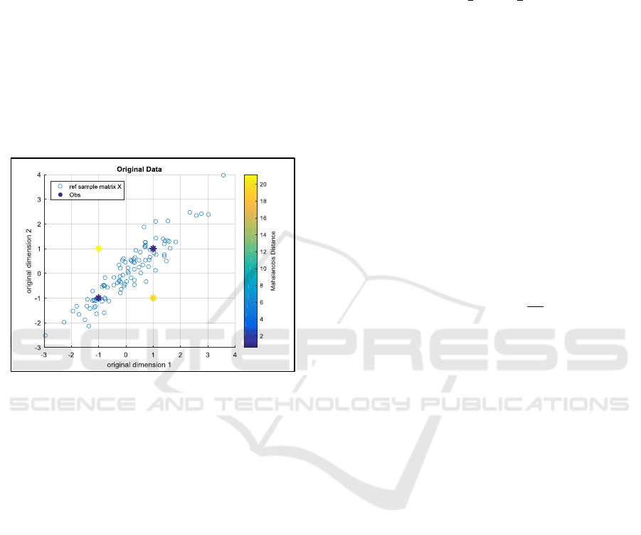
between 2 points is inappropriate. E.g., on the Figure
1, we generate synthetic centered correlated data in a
2D space (blue circles). One can see that probably the
blue stars and the data are coming from the same
distribution, whereas it is much less likely for the
yellow stars.
By using Euclidean distance, with respect to the
centre of the data (0, 0), the 4 stars would be at the
same distance (√2). Therefore ED is not appropriate
to measure distance between points and detect
outliers.
Figure 1: Synthetic data.
This is why Mahalanobis distance (MD) (De
Maesschalck et al., 2000), (Li et al., 2011) was
introduced. The idea was to de-correlate the data
before computing a Euclidean distance.
Let x
i
be an instance (1xp) in the original space, µ
the mean vector (1xp) of the p predictors and C the
covariance matrix of the data X. The squared
Mahalanobis distance
is defined by:
(2)
It measures how many variances away, the
instance is from the centre of the cloud.
Now we are going to demonstrate how MD is
linked to PCA.
Let V be the diagonal p*p matrix, such as
diag(V)=diag(C) (i.e. with the variance of each
predictor in the original space on the diagonal), and
let M be the Nxp matrix with identical row equal to
µ.
The normalized matrix X
n
can be rewritten:
(3)
And for the particular instance i:
(4)
From the basic properties of covariance operation
(cov(X.A+a)=A
T
.cov(X).A) and as V is diagonal, we
have:
(5)
Using (2), (3), (4) and (5), we get
(6)
Let y
i
be the particular instance i in the PC space.
From (1), we have
(7)
and
(8)
Using (6), (7), (8), it comes
(9)
Let y
i,j
be the j
th
component of y
i
. (9) can be
rewritten as:
(10)
The Mahalanobis distance appears to be, in the PC
space, a simple sum of squares weighted by the
inverse of variances on each PC.
Finally, in a similar way to the original space, it is
interesting to define a normalized PC space, in which
the data Y
n
are:
(11)
Using the same reasoning, it comes that the
covariance matrix of Y
n
is the identity matrix and that
the Mahalanobis distance is simply equal to the
Euclidean distance in the normalized PC space.
(12)
Which can be rewritten:
(13)
In conclusion, there are 4 different spaces: the
original one (X), the normalized one (X
n
), the PC
space (Y) and the normalized PC space (Y
n
). Each
space is defined from the previous by a simple
operation (translation, stretching and rotation) – see
equations (3), (1) and (11). In each of these spaces,
the Mahalanobis distance can be expressed, see
equations (2), (6), (9) and (12). The writing is more
or less complex, depending on the covariance matrix.
The last writing, in the normalized PC space is the
simplest and is interesting because it is a simple ED.
VEHITS 2018 - 4th International Conference on Vehicle Technology and Intelligent Transport Systems
38

The outlier detection procedure is therefore:
Run a PCA and get D, P and Y.
Using (11) project the data in the normalized
PC space, and compute for each instance the
MD using the simple ED (12).
An instance will be considered as an outlier
if its MD (or its squared MD) is above a
given threshold t:
.
The choice of the threshold t is not straightforward
and could be sometimes arbitrary. It may be helpful
to compute and plot the empirical cumulated
distribution function of the squared MD.
Once the outliers detected, it becomes possible to
identify which components are responsible for the
instances being classified as outliers. This can be
done by computing a normalized contribution of each
principal component (j=1..p) to the squared MD (14)
and looking if some components are more important
than the others:
(14)
Once some particular components have been
identified, it is sometimes possible to come back to
the original space (see the application example 3.2.1).
2.2.3 Checking Linear Dependency Between
Features
PCA helps to reveal the sometimes hidden, simplified
structures that underlie the data; an extreme case is
the linear dependency between features. In that
situation, the p
th
eigenvalue is very small D
pp
≈0,
meaning that the data projected on the associated
Principal Component p
p
have almost no variance;
using the fact that data are centered, this implies that:
(15)
p
p
represents the linear combination of the data in
normalized space. If we want to come back to the
original space, we use (3) and define a new (px1)
vector:
(16)
Such as
(17)
Therefore, the vector q
p
represents the linear
combination of the data in the original space.
2.2.4 Dimension Reduction
The most popular use of the PCA is to find the dimen-
sion of the data and/or reduce the dimension without
losing too much variance. The idea is to compute the
cumulated variance v
k, k=1..p
in the PC space:
(18)
And determine when its normalized value w
k
(19)
exceeds a given threshold t (between 0 and 1); let q
be the number of components.
(19)
The intrinsic dimension is therefore q≤p and the
data can be represented in the PC space by only the
first q PCs.
After these three steps, outliers from the data have
been removed, linear dependency between features
has been studied and data dimension has been
reduced.
2.3 Linear Discriminant Analysis
Linear Discriminant Analysis (LDA) is also called
Fisher Linear Discriminant (FDA) (Duda et al., 2001)
or Fisher Score (Gu et al., 2012). Contrary to PCA, it
is a supervised technique, which given some data,
searches for a linear combination of original variables
that best discriminates among classes (rather than best
describe the data as with PCA).
In the following, we will summarize the LDA
implementation and present an interesting
applications: feature selection.
2.3.1 LDA Implementation
Let us define some notations:
X: data in the original space, a matrix Nxp,
with N instances and p predictors.
K: number of different classes
D
k
: the subset of samples belonging to class
k,
n
k
: cardinal of D
k
m
k
: the p-dimensional mean of samples of
D
k
.
m: the p-dimensional mean of all samples.
The implementation is the following:
Compute the within-class scatter matrix S
W
which is the sum of scatter matrices S
k
:
(20)
(21)
Compute the between-class scatter matrix
S
B
:
Data Mining Applied to Transportation Mode Classification Problem
39

(22)
One can show that the total scatter matrix S
T
defined by (23) is the sum of S
W
and S
B
.
(23)
Solve for the eigenvalues and the
eigenvectors of S
W
-1
S
B
matrix; it leads to p
eigenvectors c
j, j=1..p
and p eigenvalues e
j,
j=1..p
. It can be shown S
B
is of rank K-1 at
most; therefore, there are K-1 nonzero
eigenvalues at most.
The eigenvectors, also called discriminant
axis, are linear combination of original
vectors and define a new ‘C space’ that
maximizes the class separability.
Let define a separability criteria SC as the
sum the eigenvalues (also equal to
tr(S
W
-1
S
B
). It gives an idea of how well the
classes are separated in the new C space.
Tr
(24)
2.3.2 LDA for Feature Selection
LDA is very useful for feature selection. Given a set
of p features,
We apply the LDA procedure and get an
initial separability criteria SC
0
.
We remove each feature j=1..p one by one
and compute the new separability criteria
SC
j
and the impact on class separability
r
j
=1- SC
j
/SC
0
.
We remove features whose impact is low,
i.e. |r
j
| below a threshold (typ. 0.05).
3 RESULTS
In a first section, we present the data relative to the
transportation mode problem.
Then, we apply the proposed approach.
3.1 The Data
Details about data collection, data pre-processing and
feature extraction are given in (Lorintiu and Vassilev,
2016).
A smartphone application for Android based
smartphones was developed to perform the data
collection. The application stores the raw sensor data
such as GPS, accelerometer and magnetometer. The
subjects were asked to install the developed
application on a compatible smartphone and use it
during their commute to work or any other trip. They
were also asked to choose the travel mode they are
using during the recording process. The subjects
weren’t imposed any position for their smartphone.
22 subjects participated to the database setup,
using 12 different smartphones. About 400 trips were
recorded, representing 225 hours of recording.
Three sensors, ACC, MAG and GPS were taken
into account. From the raw sensor data, signals were
segmented using a 5 seconds non overlapping
window, leading to an initial number N
I
= 161489
instances. On each window, a pre-processing was
applied to ACC whose steps are:
Estimate gravity, and subtract it from
acceleration measured, leading to the linear
acceleration
Decompose the linear acceleration into a
vertical acceleration APV and a horizontal
one APH,
Decompose the horizontal acceleration APH
into a longitudinal (or forward) H1 and a
lateral H2 acceleration.
Then, 14 a priori relevant features were computed
(see Table 1). Note that the 4 features whose name
starts with ‘ACC_V_BAND’ are defined so their sum is
equal to 1.
Table 1: The 14 features.
Seven different transportation modes were
considered: ‘bike’, ‘plane’, ‘rail’, ‘road’, ‘run’, ‘still’,
‘walk’. An additional class named ‘other’ contains
activities that are irrelevant for this study.
‘rail’ class regroups transportation modes such as
tramway, subway, train and high speed train, whereas
‘road’ assembles transportation modes such as ‘car’
and ‘bus’.
It is important to note that GPS sensor is
unavailable 42.3% of the time, representing 68316
(resp. 93173) instances unavailable (resp. available).
This quite surprising result can be explained by the
fact that as GPS is a sensor that relies on a radio wave
communication with a set of satellites, the quality of
this communication depends on
ID Name Unit Description
1 MAG_NORM_STD µT Standard deviation of magnetic field norm
2 ACC_STD_V m/s² Standard deviation of APV
3 ACC_STD_H1 m/s² Standard deviation of H1
4 ACC_STD_H2 m/s² Standard deviation of H2
5 ACC_V_BAND_EN_1 - Relative energy of APV in the band [0.7-3.5 Hz]
6 ACC_V_BAND_EN_2 - Relative energy of APV in the band [3.5-8.5 Hz]
7 ACC_V_BAND_EN_3 - Relative energy of APV in the band [8.5-18.5 Hz]
8 ACC_V_BAND_EN_4 - Relative energy of APV in the band [18.5-45 Hz]
9 ACC_SPEC_CENTROID_V Hz Spectral centroid of APV
10 MAG_SPEC_CENTROID Hz Spectral centroid of magnetic field norm
11 ACC_SPEC_SPREAD_V Hz² Spectral spread of APV
12 MAG_SPEC_SPREAD Hz² Spectral spread of magnetic field norm
13 GPS_SPD_MED m/s Median of GPS speed
14 ACC_NORM_VAR (m/s²)² Variance of accelerometer norm
VEHITS 2018 - 4th International Conference on Vehicle Technology and Intelligent Transport Systems
40
the GPS receiver sensitivity (often poor for
low cost GPS chip embedded in mobile
devices),
Radio wave attenuation due to aircraft or
train cabin or car body.
Relative position of satellites with respect to
the GPS receiver.
3.2 Application of PCA on the Data
3.2.1 Detecting Outliers
Given the available data (93173 instances), after
removing the 6615 irrelevant annotations (e.g.,
instances corresponding to ‘other’ annotations), it
remains 86558 instances.
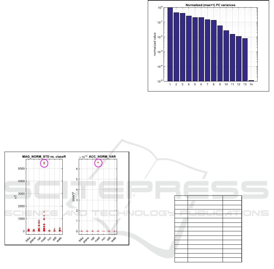
Sensor readings can be erroneous, leading to non-
physical value; below, on a 1D scatterplot (see Figure
2), it is easy to see 3 outliers, 2 relative to
MAG_NORM_STD (above 5000 µT) and one
relative to ACC_NORM_VAR (>6e12 m²/s
4
).
Figure 2: Outliers due to erroneous sensor readings.
It is very important to remove these 3 evident
outliers because, otherwise they would have distorted
the computation of mean and standard deviation when
normalizing the data for PCA computation.
Out of the 86555 remaining instances, some other
outliers are harder to discover, as each instance is
defined in a 14 dimensions feature space. To do so,
we applied the procedure presented in 0, i.e., running
a PCA and computing a MD.
The PCA computation leads to a 14
th
eigenvalue
~1000 times smaller than the others (see Figure 3
where the eigenvalues normalized have been plotted).
Figure 3: PCA normalized variances on the 14 features
data.
As explained in 2.2.3, this reveals a linear
dependency between features. From the linear
combination q
14
(see Table 2), given by the associated
principal component (see equation 16), we can
conclude that 4 features (ID between 5 and 8),
corresponding to relative energy of APV in different
frequency bands are linearly dependent. This is not
surprising given how these 4 features have been
computed (see 3.1).
Table 2: Linear combination of the 14 features.
Therefore, we remove one of the 4 features; we
arbitrary chose to remove the last one,
‘ACC_V_BAND_EN_4’. We run again a PCA in the
13
th
dimensional space. Figure 4 displays the matrix
P. Columns correspond to principal components and
rows to features (The “_N” added at the end of each
feature name reminds that the PCA is done on
normalized data). We can see, e.g., that the 2
nd
PC
(column 2) involves mainly the 2 features,
‘MAG_SPEC_CENTROID’ and ‘MAG_SPEC_SPREAD’
which are the relative spectral energy of the magnetic
field.
ID Name
q
14
1 MAG_NORM_STD 0.000
2 ACC_STD_V 0.000
3 ACC_STD_H1 0.000
4 ACC_STD_H2 0.000
5 ACC_V_BAND_EN_1 2.174
6 ACC_V_BAND_EN_2 2.174
7 ACC_V_BAND_EN_3 2.174
8 ACC_V_BAND_EN_4 2.174
9 ACC_SPEC_CENTROID_V 0.000
10 MAG_SPEC_CENTROID 0.004
11 ACC_SPEC_SPREAD_V 0.000
12 MAG_SPEC_SPREAD 0.000
13 GPS_SPD_MED 0.000
14 ACC_NORM_VAR 0.000
Data Mining Applied to Transportation Mode Classification Problem
41
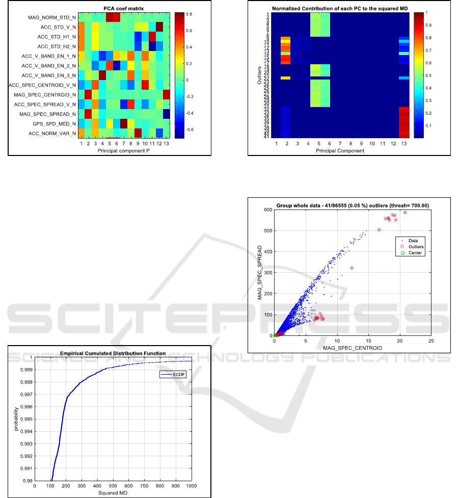
Figure 4: Principal Components on the 13 features data.
Then, for each of the 86555 instances, we
compute the squared MD according to equations 11
and 12.
Considering the empirical cumulated distribution
function of the squared MD (Figure 5), we decided to
set a relatively high threshold (equal to 700) in order
to remove a small number of outliers.
For the resulting 41 outliers, we compute the
normalized contribution of each principal component
to the squared MD (see equation 14). Figure 6 shows
2 distinct groups of outliers, the first one due to high
values on components 2 and 13, the 2
nd
one due to
high values on components 5 and 6.
Figure 5: Empirical cumulated distribution function of
the squared MD.
Regarding the 1
st
group, Figure 4 shows that
principal components 2 and 13 involve mainly the
two previously mentioned features relative to spectral
energy of the magnetic field. Plotting the outliers in
this 2D space is therefore relevant as Figure 7 shows
it.
Figure 6: Normalized contribution of each PC to squared
MD for the 41 outliers.
Figure 7: 41 outliers displayed in a 2D original space.
This procedure to automatically locate the outliers
can be applied either on the global dataset, as it has
been done, or for each of the seven classes. It leads to
the removal of a total of 504 outliers.
The last source of outliers was wrong user
annotation. E.g., each time the subject was moving
and stopped for any reason (for e.g., when walking to
look to a map, or to wait for the red-light, or in a train
that stops at a station), the user annotation should be
changed to ‘still’; obviously, we could not ask the
volunteer to do so, because it would have been too
cumbersome. The consequence is that some instances
are not correctly annotated. After checking the
instances thanks to the GPS speed, we discard 3251
outliers; most are due to walking at very low speed
(<1 km/h).
Finally, after removing the different outliers
(3+504+3251), it remains 82000 instances, i.e. 89%
of the 93173 original instances.
VEHITS 2018 - 4th International Conference on Vehicle Technology and Intelligent Transport Systems
42
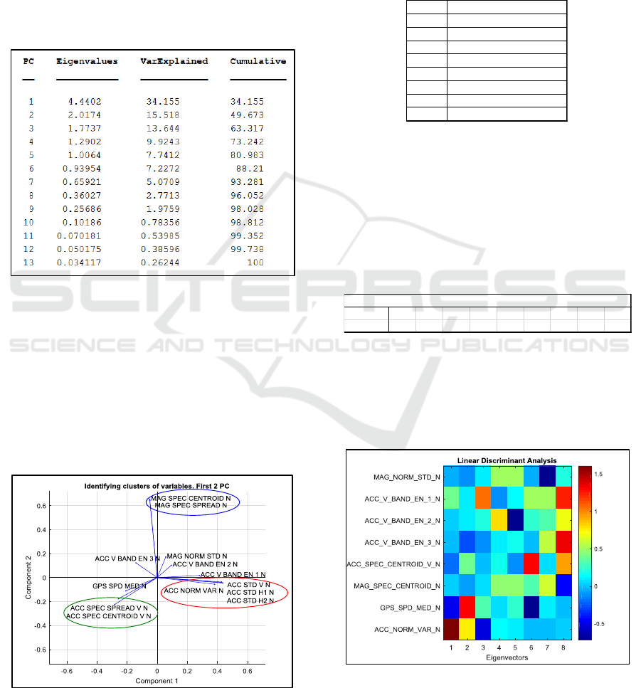
3.2.2 Dimension Reduction
After the outliers were removed, a 3
rd
and last PCA
was performed. Eigenvalues are displayed in the 2
nd
column of Table 3. The 3
rd
column corresponds to the
ratio between each eigenvalue and the sum of the
eigenvalues in percentage. Finally, the last column is
the cumulated sum of the previous one. This table
shows that 8 components explains 96 % of the
variance of the data.
Table 3: Eigenvalues.
Therefore the dimension of the data can be
reduced from 13 to 8 and the next steps, such as
classifier training could be done on the 8 components
in the PC space: p
1
, p
2
, …, p
8
. But working with data
in the PC space is less intuitive and more complex.
This is why, it is often better practice, if possible, to
remove original variables. To do so, we focussed on
the first 2 columns of the P matrix. In Figure 8, each
of the 13
th
original variables was plotted with a blue
line starting from the origin, in the 2D plane formed
by the first 2 PCs.
Figure 8: Identifying clusters of original variables.
Three main clusters stick out from Figure 8 (resp.
displayed in red, blue and green), with resp. 2, 2 and
4 features.
Therefore, one feature by cluster can be kept,
removing 1+1+3=5 features. The problem could
therefore be simplified to 8 dimensions. Table 4
summarizes the 8 features finally kept.
Table 4: 8 features after dimension reduction.
3.3 Application of LDA on the Data
We apply a LDA on the database obtained after PCA
application (see 3.2), which has 82800 samples and 8
features. Among the 8 eigenvalues, 6 are non-null
(see Table 5). For this nominal configuration, the
separability criteria is 5.05.
Table 5: Eigenvalues of the LDA.
Figure 9 presents the 8 eigenvectors (in column)
which are linear combination of the 8 original
variables (in row). E.g., the first eigenvector, i.e. the
vector that best linearly separates the classes appears
to be a combination of the GPS speed and the
accelerometer variance.
Figure 9: Eigenvectors.
In this case, it is also meaningful to represent the
data in the 2D spaced formed the first two
ID Name
1 MAG_NORM_STD
2 ACC_V_BAND_EN_1
3 ACC_V_BAND_EN_2
4 ACC_V_BAND_EN_3
5 ACC_SPEC_CENTROID_V
6 MAG_SPEC_CENTROID
7 GPS_SPD_MED
8 ACC_NORM_VAR
ID 1 2 3 4 5 6 7 8 Sum
Eigenvalue 3.00 1.60 0.19 0.17 0.08 0.01 0.00 0.00 5.05
LDA - Eigenvalues
Data Mining Applied to Transportation Mode Classification Problem
43
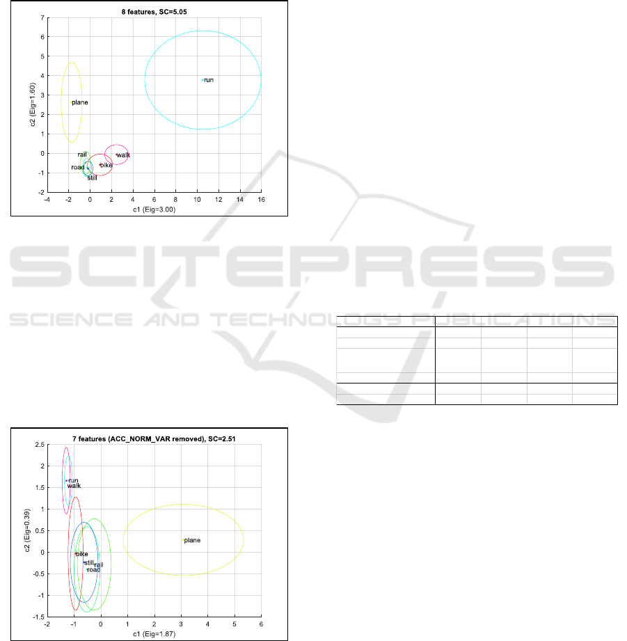
eigenvectors. As there may be confusions between
some classes, instead of plotting each sample, we
draw, for each class an ellipse representing the
dispersion. The ellipse’s centre stands for the mean,
whereas the semi axis length is equal to the standard
deviation. On Figure 10, one can see, that ‘run’ and
‘plane’ are well separated in this space, whereas there
is some confusion between ‘bike’ and ‘walk’ and
even more confusion between the 3 remaining classes
‘rail’, ‘road’ and ‘still’.
Figure 10: Class separability with 8 features.
Now, if we remove one feature, e.g.
‘ACC_NORM_VAR’, and do again a LDA, we get a new
set of eigenvectors and eigenvalue. Compared to the
previous nominal configuration, the separability
criteria highly decreases to 2.51 (-50%). Figure 11 is
a good illustration: ‘plane’ is still an isolated class
(thanks to the GPS speed), but it is no more the case
for ‘run’ which is now confused with ‘walk’. We can
conclude that ‘ACC_NORM_VAR’ is an important
feature.
Figure 11: Class separability with 7 features
(ACC_NORM_VAR removed).
On the contrary if we remove the feature
‘MAG_NORM_STD’, the separability criteria is very few
changed: 4.97, compared to 5.05.
3.4 Validation
To validate the results obtained after the previous
processing, we considered the 82000 instances
database obtained after outliers’ removal. We built 4
classification models (M1, M2, M3 and M4), the first
one M1 using the 13 features, M2 the 8 ones after
dimension reduction, M3 and M4 7 features. In M3,
with respect to M2, we removed one feature:
‘ACC_NORM_VAR’, whereas in M4 we removed
‘MAG_NORM_STD’.
These classifiers were all based on decision trees
constrained by a maximum number of splits of 32
(this figure represents a good compromise between
classifier’s performance and complexity).
Performance assessment for each model is done
via a Leave-One-Subject-Out Cross Validation
(LOSO CV) procedure (Arlot and Celisse, 2010),
which involves the partition of the database into K
folds, each fold representing a subject. The
performance metric used is the F-measure (harmonic
mean of precision and recall) averaged over the
different classes.
The results are summarized in Table 6.
Table 6: performance for the different models.
Comparing M1 and M2, it appears that reducing
the dimension using a PCA even improves the
performance: 0.714 instead of 0.689, i.e. +0.025. This
can be explained by the fact that removing 5 features
might have simplified the problem.
Comparing M3 and M4 with respect to M2 shows
that the separability criteria seems to be a good
indicator of the importance of a feature and its impact
on classification performance; so, removing
‘ACC_NORM_VAR’ reduces SC by 50% and
performance drops by ~0.1 whereas removing
‘MAG_NORM_STD’ decreases only slightly the SC
(-1.6%) and performance (-0.01).
The resulting decision trees have a number of
nodes comprised between 53 and 61, which is too
high if one wants to display the trees. Nevertheless,
comparing them shows that M2 and M4 are quite
similar (their 2 most important variables are
M1 M2 M3 M4
Number of predictors 13 8 7 7
Predictor removed w.r.t M2 ACC_NORM_VAR MAG_NORM_STD
Important variables
ACC_STD_V,
ACC_NORM_VAR,
GPS_SPD_MED
ACC_NORM_VAR,
GPS_SPD_MED
GPS_SPD_MED
ACC_NORM_VAR,
GPS_SPD_MED
Performance (Avg. F-measure) 0.689 0.714 0.612 0.703
Separability Criteria (SC) 5.05 2.51 4.97
impact on SC -50.3% -1.6%
VEHITS 2018 - 4th International Conference on Vehicle Technology and Intelligent Transport Systems
44

ACC_NORM_VAR and GPS_SPD_MED), whereas the
other 2 models M1 and M3 are different: M1 differs
because it involves ACC_STD_V which brings the same
information as ACC_NORM_VAR. M3 differs because it
does not have access to ACC_NORM_VAR.
4 CONCLUSIONS
Given a classification (or regression) problem, due to
the number of different possible combinations of
sensors, features, classifiers and hyper-parameters,
finding an optimal classifier is a very time consuming
task.
This is why, simplifying the problem, using quick
data mining tools is very interesting.
In this study, we present three simple data mining
tools: Principal Component Analysis, Mahalanobis
distance and Linear Discriminant Analysis.
We apply them on real data concerning the
transportation mode classification problem and show
that we are able to
clean the data: we remove outliers
representing 11% of the samples
simplify the problem: we reduce data
dimension from 14 to 8 and this
simplification even improves the classifier
performance
study the importance of each of 8 features;
it turns out that feature ‘ACC_NORM_VAR’ is
very important whereas ‘MAG_NORM_STD’ can
be removed with a small effect on
performance (-0.01).
ACKNOWLEDGEMENTS
This work is part of the BONVOYAGE project which
has received funding from the European Union’s
Horizon 2020 research and innovation programme
under grant agreement No 635867.
REFERENCES
Anderson, I., Muller, H., 2006. Exploring GSM Signal
Strength Levels in Pervasive Environments, in: 20th
International Conference on Advanced Information
Networking and Applications, 2006. AINA 2006.
Presented at the 20th International Conference on
Advanced Information Networking and Applications,
2006. AINA 2006, pp. 87–91. https://doi.org/10.1109/
AINA.2006.176
Arlot, S., Celisse, A., 2010. A survey of cross-validation
procedures for model selection. Stat. Surv. 4, 40–79.
https://doi.org/10.1214/09-SS054
De Maesschalck, R., Jouan-Rimbaud, D., Massart, D.L.,
2000. The Mahalanobis distance. Chemom. Intell. Lab.
Syst. 50, 1–18. https://doi.org/10.1016/S0169-
7439(99)00047-7
Duda, R.O., Hart, P.E., Stork, D.G., 2001. Pattern
Classification by Richard O. Duda, David G. Stork,
Peter E.Hart .pdf.
Gu, Q., Li, Z., Han, J., 2012. Generalized fisher score for
feature selection. ArXiv Prepr. ArXiv12023725.
Hemminki, S., Nurmi, P., Tarkoma, S., 2013.
Accelerometer-based Transportation Mode Detection
on Smartphones, in: Proceedings of the 11th ACM
Conference on Embedded Networked Sensor Systems.
ACM, New York, NY, USA, p. 13:1–13:14.
https://doi.org/10.1145/2517351.2517367
Li, C., Georgiopoulos, M., Anagnostopoulos, G.C., 2011.
Kernel principal subspace Mahalanobis distances for
outlier detection, in: The 2011 International Joint
Conference on Neural Networks. Presented at the The
2011 International Joint Conference on Neural
Networks, pp. 2528–2535. https://doi.org/10.1109/
IJCNN.2011.6033548
Lorintiu, O., Vassilev, A., 2016. Transportation mode
recognition based on smartphone embedded sensors for
carbon footprint estimation, in: 2016 IEEE 19th
International Conference on Intelligent Transportation
Systems (ITSC). Presented at the 2016 IEEE 19th
International Conference on Intelligent Transportation
Systems (ITSC), pp. 1976–1981. https://doi.org/
10.1109/ITSC.2016.7795875
Manzoni, V., Maniloff, D., Kloeckl, K., Ratti, C., 2010.
Transportation mode identification and real-time CO2
emission estimation using smartphones.
Martinez, A.M., Kak, A.C., 2001. PCA versus LDA. IEEE
Trans. Pattern Anal. Mach. Intell. 23, 228–233.
https://doi.org/10.1109/34.908974
Nitsche, P., Widhalm, P., Breuss, S., Brändle, N., Maurer,
P., 2014. Supporting large-scale travel surveys with
smartphones – A practical approach. Transp. Res. Part
C Emerg. Technol. 43, 212–221. https://doi.org/
10.1016/j.trc.2013.11.005
Reddy, S., Mun, M., Burke, J., Estrin, D., Hansen, M.,
Srivastava, M., 2010. Using Mobile Phones to
Determine Transportation Modes. ACM Trans Sen
Netw 6, 13:1–13:27. https://doi.org/10.1145/1689239.
1689243
Sankaran, K., Zhu, M., Guo, X.F., Ananda, A.L., Chan,
M.C., Peh, L.-S., 2014. Using Mobile Phone Barometer
for Low-power Transportation Context Detection, in:
Proceedings of the 12th ACM Conference on
Embedded Network Sensor Systems. ACM, New York,
NY, USA, pp. 191–205. https://doi.org/10.1145/
2668332.2668343
Stenneth, L., Wolfson, O., Yu, P.S., Xu, B., 2011.
Transportation Mode Detection Using Mobile Phones
and GIS Information, in: Proceedings of the 19th ACM
SIGSPATIAL International Conference on Advances
Data Mining Applied to Transportation Mode Classification Problem
45

in Geographic Information Systems. ACM, New York,
NY, USA, pp. 54–63. https://doi.org/10.1145/2093973.
2093982
Vlahogianni, E.I., Barmpounakis, E.N., 2017. Driving
analytics using smartphones: Algorithms, comparisons
and challenges. Transp. Res. Part C Emerg. Technol.
79, 196–206. https://doi.org/10.1016/j.trc.2017.03.014
Wikipedia, 2017. Principal component analysis. Wikipedia.
Wu, L., Yang, B., Jing, P., 2016. Travel mode detection
based on GPS raw data collected by smartphones: A
systematic review of the existing methodologies. Inf.
Switz. 7. https://doi.org/10.3390/info7040067
VEHITS 2018 - 4th International Conference on Vehicle Technology and Intelligent Transport Systems
46
