
Adaptive Cruise Control for Electric Bus based on Model Predictive
Control with Road Grade Prediction
Jindong Bian, Bin Qiu, Yahui Liu and Haotian Su
State Key Laboratory of Automotive Safety and Energy, Tsinghua University, Haidian District, Beijing, China
Keywords: Adaptive Cruise Control, Model Predictive Control, Road Grade Prediction, Electric Bus.
Abstract: Adaptive Cruise Control (ACC) makes the driving experience safer and more pleasurable. To
comprehensively deal with tracking capability and energy consumption issue of ACC-activated vehicle on
rugged roads, this paper presents a MPC based vehicular following control algorithm with road grade
prediction. A simulation model of ACC for electric bus based on MPC is built for analysing the
performance of the algorithm. The simulation results show that road grade prediction can improve improves
both energy consumption and tracking capability.
1 INTRODUCTION
Cruise Control (CC) executes the task of
maintaining the vehicle speed at a desired value.
However, it cannot reasonably alter the speed of the
vehicle according to different situations. When the
preceding vehicle equipped with CC is traveling
slower than the latter, the driver has to step on the
brake pedal in order to deactivate the Cruise Control
and step on the accelerator when the preceding
vehicle speeds up, (Howard, 2013). This drawback
is overcome by the more advanced Adaptive Cruise
Control (ACC), which is able to adjust the vehicle
speed by analysing various influential factors,
without manual intervention from the driver,
(Howard, 2013; Shakouri et al., 2012, 2014).
Adaptive Cruise Control system (ACC) has been
widely investigated due to its merits of reducing
driver workload and ensuring safety, (Mba et al.,
2016). Due to concerns about global warming and
energy conservation, vehicle energy consumption
has become a consideration of great importance for
the automotive industry. Close attention has been
given to another important issue in ACC,
specifically energy consumption problem, (Li et al.,
2017). Tsugawa and Ioannou suggested the use of
ITS technologies, including adaptive cruise control,
to reduce fuel consumption of vehicles, (Tsugawa,
2001; Ioannou et al., 2005; Bose et al., 2003). ACC
system is designed to follow the vehicle in front
automatically, simultaneously to reduce energy
consumption to the full extent under the premise of
ensuring safety. The design of an ACC system with
multiple objectives can be naturally cast into a
model predictive control (MPC) framework. MPC
has already proved its merit in ACC design in
literature, (Li et al., 2011). Nonetheless, ACC
system based on MPC designed for conventional
fuel vehicles is not suitable for electric buses which
are equipped with regenerative braking system.
When taken into account, the road grade effect
can play an important role in advanced navigation
and navigation algorithms, where the system can
help drivers avoid steep roads to achieve better fuel
economy and reduce carbon dioxide emissions,
(Boriboonsomsin et al., 2009). A research has found
that fuel saving capability of ACC system can be
strenthened by the prediction of road grade,
(Lattemann et al., 2009). Knowledge about the
upcoming road grade can be used in ACC to avoid
unnecessary braking and shifting. Due to the
relatively large mass of a city bus, such system can
save a great deal of energy. In addition, road grade
level has an effect on crash risk, (Wu et al., 2017).
Therefore, if in the future road grade can be
accurately predicted, the valuable data can reduce
not only the energy consumption of buses, but also
the risk of traffic accidents, (Zeng et al., 2015; Luo
et al., 2015).
There are many methods to measure or estimate
the current road slope during driving, (Kim et al.,
2013). These methods generally rely on different
types of sensors, mainly Global Position System
Bian, J., Qiu, B., Liu, Y. and Su, H.
Adaptive Cruise Control for Electric Bus based on Model Predictive Control with Road Grade Prediction.
DOI: 10.5220/0006641702170224
In Proceedings of the 4th International Conference on Vehicle Technology and Intelligent Transport Systems (VEHITS 2018), pages 217-224
ISBN: 978-989-758-293-6
Copyright
c
2019 by SCITEPRESS – Science and Technology Publications, Lda. All rights reserved
217

(GPS), inertial sensors, pressure sensors, (Boroujeni
et al., 2013), wheel speed sensors, (Wragge-Morley
et al., 2013), acceleration sensors, LIDAR, (Tsai et
al., 2013), etc. GPS can provide the altitude and
velocity information of the vehicle, but the signal
accuracy is greatly influenced by the environment.
GPS cannot provide reliable data in conglomerations
of high-rise buildings and inside tunnels and so on,
(Bae et al., 2001). IMU (Inertial Measurement Unit)
can provide acceleration and angular velocity
information and is not affected by environment
factors. However, its measurement accuracy can be
easily influenced by suspension movements, and its
signal oscillation can be very serious, (Lee et al.,
2012). Based on prior analysis, researchers have
proposed some methods and algorithms to improve
the accuracy of road slope estimation, such as
Kalman filter, extended Kalman filter, (Srinivasaiah
et al., 2014), etc.
This paper is organized as follows. The second
part introduces the longitudinal vehicle dynamics.
The third part introduces the MPC algorithm in this
paper, including the state space description of the
problem and the construction of cost function. The
fourth part introduces the road grade prediction. A
simulation model and results are shown in the fifth
part, indicating the improvement of ACC based on
MPC with road grade consideration.
2 LONGITUDINAL VEHICLE
DYNAMICS
Figure 1 shows the schematic diagram of an electric
bus’s longitudinal model, where
accl
a
represents
the acceleration pedal position,
brk
a
is brake pedal
position,
a
F
is aerodynamic drag,
f
F
is rolling
resistance and
i
F
is climbing resistance. The motor
torque is mainly affected by the accelerator pedal
signal and the motor speed. Compared with
traditional vehicles, most electric vehicles are
equipped with a regenerative braking system, which
can recover energy while braking.
Motor
Brake System
Driver
Train
Vehicle Body
Motor Torque
Regenerative Brake Torque
Vehicle Speed
Friction Brake Torque
a
F
f
F
i
F
v
Drive Torque
accl
a
brk
a
Figure 1: Longitudinal dynamics of electric bus.
3 ACC ALGORITHIM BASED ON
MPC
3.1 Discrete State Space Model
With respect to inter-vehicular dynamics, we define
two variables reflecting the tracking errors:
clearance error ∆d and speed error ∆v. The discrete
state space model can be described as:
22
( 1) ( ) ( ) ( )
( ) ( )
,
[ ] , ,
0. 5 0. 5
1
,,
01
[]
des p f
f des p
cc
c
cc
mm
x k Ax k Bu k G k
y k Cx k
d d d v v v
x d v u a a
TT
T
A B G
TT
y d v
(1)
where C is identity matrix,
c
T
is the sample
time, d is distance between two vehicles,
des
d
is
desired distance,
p
v
is the preceding vehicle speed,
f
v
is the following vehicle speed,
p
a
is the
preceding vehicle acceleration,
fdes
a
is the needed
acceleration of following vehicle. For a typical ACC
system, radar and accelerometer are equipped, which
means the states are measurable.
3.2 Construction of Optimization
Problem
Tracking capability, fuel economy, driver behaviour,
driving safety, ride comfort and environmental
issues, as well as limitations on the model and traffic
flow, all of the above factors constrain the behaviour
of the ACC system. In this paper, emphasis is given
to energy consumption and tracking capability while
allowing driver permissible tracking error.
According to MPC framework, the cost function
to be optimized can perform a trade-off between the
former two issues since they are reversely interactive
with each other. Driver permissible tracking error
issue mainly results from driver behaviour in actual
traffic flow. If inter vehicular distance is larger, the
cut-in of front vehicle from adjacent lane occurs
frequently, thus leading to frequent decelerating of
ego car and the deterioration of fuel economy. On
the other hand, if the distance is smaller, driver is
prone to intervene ACC control to avoid potential
VEHITS 2018 - 4th International Conference on Vehicle Technology and Intelligent Transport Systems
218

rear-end collision. Both strategies are sure to disturb
ACC’s regular working order. So, the upper and
lower bounds of tracking errors usually exist, called
the driver permissible tracking error.
Fine tracking capability does not mean that the
energy consumption is optimal. ACC system
designed for the electric bus is different from the one
of traditional fuel vehicles. Because of the existence
of regenerative braking system, the energy
consumption cannot be simply regarded as the linear
function of the squared value of the acceleration. An
energy consumption model of electric bus is
established as follow:
3
cos si n
( , ) ( )
3600 3600 76140 3600
D
wh f f des f f f f des
CA
Gf G m
P v a v v v a
(2)
,0
0, 0
,
(1 ) , 0
0, 0
wh
wh
wh
Td Md
req req
wh Tb Mb el c wh
wh
P
P
P
PP
PP
P
(3)
where α is the road gradient and while the vehicle is
downhill, the value of α is negative, f is the rolling
resistance coefficient, m is the vehicle mass,
D
C
is the coefficient of air resistance that is
characterized by the shape of the vehicle’s body,
f
v
is the vehicle speed, δ is a coefficient that
characterizes the rotational inertia of the vehicle, A
is the windward area,
Td
and
Tb
are the
powertrain efficiency,
Md
and
Mb
are the motor
efficiency, β is the ratio of front-rear braking force
allocation,
elc
is the regenerative braking force
coefficient. The cost function of MPC is established
as:
2
11
mi n ( ( ) ( ) ) ( )
PP
req req
kk
J K P k P k L d k
(4)
max
mi n max
mi n max
()
0 ( )
( ) (1 )
()
()
el cb
el c
wh Tb M
f des f des f des
Pk
k
Pk
a a k a
d d k d
(5)
3
max
max
mi n
cos si n
()
( ) ( )
(1 )
3600 3600 76140
3600
D
el cb
hydb f f
Tb M el c
f des
f
CA
Gf G
Pk
P k v v
a
m
v
(6)
3
max
max
cos si n
( ) ( )
3600 3600 76140
3600
D
el cd T M f f
f des
f
CA
Gf G
P k v v
a
m
v
(7)
where P is the control horizon, K and L are the
weight coefficients,
maxelcb
P
is the maximum
regenerative braking power and
maxelcd
P
is the
maximum driving power, which depends on the
motor and the battery.
maxhydb
P
is the maximum
hydraulic braking power.
Pseudo-spectral (PS) is an effective numerical
method for solving optimal control problem (OCP).
It uses the zeroes of orthogonal polynomials as
collocations, and uses global interpolation to
approximate the original continuous variables, and
transforms the OCP into a nonlinear programming
problem (NLP). And there are a variety of mature
and effective methods for solving NLP, (Elnagar et
al., 1995). Compared with other traditional methods,
PS features the high precision and fast convergence,
(Xu et al., 2015), so this paper chooses PS as the
tool for solving MPC optimization problems.
4 ROAD GRADE PREDICTION
According to the longitudinal dynamics of electric
bus, without road grade taken into account in ACC,
Adaptive Cruise Control for Electric Bus based on Model Predictive Control with Road Grade Prediction
219
the difference between
fdes
a
and
f
a
may be
beyond expectation, which may lead to safety
problems. Therefore, considering the road grade is
very meaningful for ACC, especially when the road
grade is predictable in the control period.
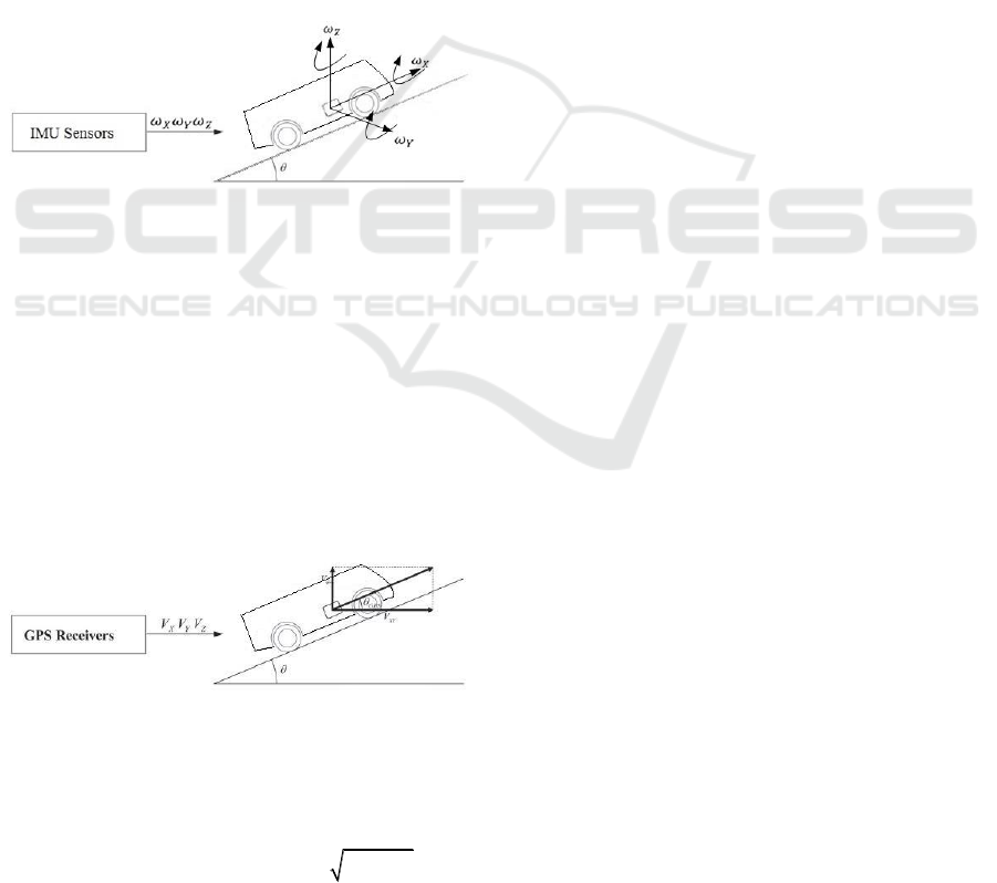
4.1 Road Grade Estimation
4.1.1 Measuring Road Slope with IMU
IMU sensors have been widely used for road slope
estimation because it can provide 3-D angular
velocity (Figure 2). The road slope can be obtained
by integrating the Y-axis angular velocity, (Wang et
al., 2013), as shown in the following:
0
0
t
I MU Y t
t
dt
(8)
Figure 2: Measuring Road Slope with IMU.
4.1.2 Measuring Road Slope with GPS
GPS receivers have been widely used for road slope
estimation because GPS provides both vehicle
altitude and velocity information in the navigation
frame. Using 3-D velocities from a GPS receiver
(Figure 3), the road slope can be estimated by
calculating the ratio of vertical velocity to horizontal
velocity, (Bae et al., 2001). By combining the
change of road altitude, the road slope measurement
is more accurate.
Figure 3: Measuring Road Slope with GPS.
The road slope can be determined by calculating
the arctangent value of the vertical velocity divided
by the horizontal velocity measurement:
1 1 2 2
t an ( / ) t an ( / )
GPS Z XY Z X Y
V V V V V
(9)
However, road slope estimation methods based
on GPS might be hampered by temporary losses of
satellite connection and multipath errors. The GPS
and IMU data are processed by Kalman filter to
estimate the current road grade.
4.1.3 Road Invariant Model
As the road is changing slowly, in a short period the
road model can be considered as:
( ) ( 1)kk
(10)
Estimating the current road slope and using the road
invariant model can predict the road grade within the
control horizon.
4.2 Data Acquisition Experiment
Driving cycles are usually used to assess the
performance of vehicles from several aspects, for
example, fuel consumption and pollution emissions.
However, conventional driving cycles like NEDC
are only series of data points representing the speed
of vehicles at different time. To take real-world road
gradient information into account in ACC,
information given by conventional driving cycles is
insufficient and road gradient data need to be added
to constitute a new driving cycle.
Two routes carefully chosen in Beijing were
traced and raw data of road gradient and velocity
were acquired simultaneously for further processing
and analysis. One route is high way which contains
some flyovers and the other route is city road which
is chosen to avoid any flyovers. The data of vehicle
speed and road grade were collected simultaneously,
which can be seen in Figure 4.
5 SIMULATION AND ANALYSIS
In order to study whether road grade has influence
on ACC, a simulation is carried out based on the
nonlinear electric bus longitudinal model. The
parameters used for simulation are given in Table 1.
VEHITS 2018 - 4th International Conference on Vehicle Technology and Intelligent Transport Systems
220
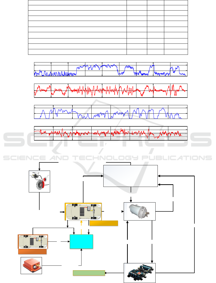
Table 1: Parameters of electric bus.
Parameters
Symbol
Unit
Value
Curb weight
M
Kg
5600
Motor power (default/ peak)
P
kW
80/130
Motor torque (default/ peak)
T
Nm
350/900
Transmission ratio
G
i
5.39
Dynamic rolling radius
r
mm
336
Aerodynamic drag coefficient
D
C
0.6
Frontal area
A
m
2
4.95
Distance of gravity centre to front wheel centre
a
L
mm
2050
Distance of gravity centre to rear wheel centre
b
L
mm
1645
0 500 1000 1500 2000 2500 3000 3500 4000 4500
0
10
20
Speed(m/s)
High Way
0 500 1000 1500 2000 2500 3000 3500 4000 4500
-0.05
0
0.05
Road Grade(rad)
0 200 400 600 800 1000 1200 1400 1600
0
10
20
Speed(m/s)
City Road
0 200 400 600 800 1000 1200 1400 1600
-0.04
-0.02
0
0.02
0.04
Road Grade(rad)
Time(sec)
Figure 4: Data of speed and road grade.
Required torque
Braking torque &
Driving torque
control
Motor torque demand
Motor speed
Required power
Available power
Available motor torque
SOC
Hydraulic braking torque demand
Hydraulic braking torque
ACC based
MPC
Vp
Vf
Road gradient
Preceding vehicle
GPS+IMU sensor
Following vehicle
Distance
Energy consumption
Afdes
Figure 5: Simulation model.
Adaptive Cruise Control for Electric Bus based on Model Predictive Control with Road Grade Prediction
221
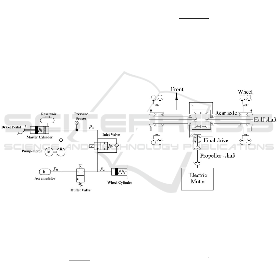
5.1 Hydraulic Brake System
A schematic diagram of a hydraulic braking system
is shown in Figure 6. The inlet valve (normally
open) and the outlet valve (normally closed) are set
upstream and downstream respectively of the wheel
cylinder.
m
p
is the master cylinder pressure, which
is the input pressure of the inlet valve and
w
p
is
the wheel cylinder pressure, which is the load
pressure in the hydraulic control system. The
structure of the wheel cylinder is simplified to a
combination of piston and spring. For an electrified
vehicle in the regenerative deceleration process,
when the driver depresses the brake pedal, the brake
pressure
m
p
will be generated in the master
cylinder, which can indicate the total brake demand
of the vehicle. The regenerative braking torque
provided by the motor will be exerted on the drive
axle. Meanwhile, to assist the overall braking
operation, the expected brake pressure
w
p
can be
obtained and applied to the wheel cylinder by
modulating the inlet valve, (Lv et al., 2017).
Figure 6: Schematic diagram of the hydraulic braking
system.
For an electric vehicle, the total braking torque
b
T
is cooperatively provided by the regenerative
braking torque and friction braking torque according
to:
4
b f b w
b G r egen hb m
rA
T i T T p
(11)
where β is set at 0.4 in this paper,
b
is the friction
coefficient of the brake disc,
m
p
is the pressure of
the master cylinder,
fb
r
is the effective friction
radius of the brake disc,
w
A
is the contact area, and
regen
T
is the regenerative braking torque.
5.2 Electric Powertrain System
The electric powertrain is shown in Figure 7, which
can be described as:
,0
,0
whdes
mm
Td G
whdes wh
m Tb m
G
Fr
TT
i
F r T
TT
i
(12)
where
m
T
is the torque of electric motor. When the
motor is on drive mode,
m
T
>0; and
m
T
<0 when the
motor works as a generator.
whdes
F
is the desired
force on wheel, r is the rolling radius of wheel,
G
i
is the transmission ratio.
Figure 7: Electric Powertrain.
5.3 Motor and Battery
According to the motor map, it is useful to find the
motor's external characteristics of torque, drive
efficiency and generation efficiency. The motor
torque is simplified as a first-order inertia system:
Mdes M M M
T T T
(13)
where
Mdes
T
is the desired motor torque,
M
T
is the
actual motor torque,
M
is time coefficient.
The battery model with the internal dissipation is
used to analyse the performance characteristics of an
electric battery. The input of the model is the
VEHITS 2018 - 4th International Conference on Vehicle Technology and Intelligent Transport Systems
222

demand power of the motor, the output is the
battery’s SOC, voltage, current and output power.
5.4 Simulation Results
In order to verify the performance of ACC,
simulation patterns for actual road conditions is
adopted here. The speed and road grade profiles are
illustrated in Figure 4. Tracking Error Index (TEI) is
composed of both speed error and distance error, (Li
et al., 2008):
1
1 ( )
()
N
k
DV
dk
TEI v k
NK
(14)
where N is length of simulation pattern,
DV
K
is
weighting coefficient, reflecting different emphasis
on ∆d and ∆v. Here, according to actual driver
experiment data, we select
DV
K
=10. The TEI
values with its corresponding energy consumption
under city road and high way simulation patterns are
shown in Table 2. With road grade taken into
consideration, in high way pattern, the TEI value is
reduced by 2.6 % while energy consumption per
100km decreases 4.9%. With respect to city road
pattern, they are 1.0% and 3.1%. A conclusion can
be drawn from Figure 4 and Table 2 that there is
greater promotion of energy consumption in high
way pattern than in city road with road grade
prediction because the high way is more varied in
altitude than the city road.
Table 2: Performance of ACC based MPC.
Simulation Pattern
TEI
Energy
Consumption
(kWh/100km)
High
Way
ACC without road
grade prediction
0.069
38.68
ACC with road
grade prediction
0.067
36.80
City
Road
ACC without road
grade prediction
0.097
41.77
ACC with road
grade prediction
0.096
40.45
6 CONCLUSIONS
In this paper, MPC is used as ACC algorithm. This
paper proposes to use Kalman filter to estimate the
current road grade with data gathered via GPS and
IMU sensor; and to use the road invariant model to
predict the road grade within the control horizon of
MPC, making possible the optimization of the track
performance and the reduction of energy
consumption. Based on the establishment of an
electric bus simulation model, and the use of
collected speed and road grade data, simulation
results verify the improvement of performance of
ACC with road grade prediction.
ACKNOWLEDGEMENTS
This research was made possible in part by the
generous support of Collaborative Innovation Centre
of Electric Vehicles in Beijing.
REFERENCES
Howard, B. (2013). What is adaptive cruise control, and
how does it work?. Extreme Tech, Electronics Section.
Shakouri, P., Ordys, A., & Askari, M. R. (2012). Adaptive
cruise control with stop&go function using the
state-dependent nonlinear model predictive control
approach. ISA transactions, 51(5), 622-631.
Shakouri, P., & Ordys, A. (2014). Nonlinear model
predictive control approach in design of adaptive
cruise control with automated switching to cruise
control. Control Engineering Practice, 26, 160-177.
Mba, C. U., & Novara, C. (2016). Evaluation and
Optimization of Adaptive Cruise Control Policies Via
Numerical Simulations.
Li, S. E., Zheng, Y., Li, K., Wu, Y., Hedrick, J. K., Gao,
F., & Zhang, H. (2017). Dynamical Modeling and
Distributed Control of Connected and Automated
Vehicles: Challenges and Opportunities. IEEE
Intelligent Transportation Systems Magazine, 9(3),
46-58.
Tsugawa, S. (2001). An overview on energy conservation
in automobile traffic and transportation with ITS. In
Vehicle Electronics Conference, 2001. IVEC 2001.
Proceedings of the IEEE International (pp. 137-142).
IEEE.
Ioannou, P. A., & Stefanovic, M. (2005). Evaluation of
ACC vehicles in mixed traffic: Lane change effects
and sensitivity analysis. IEEE Transactions on
Intelligent Transportation Systems, 6(1), 79-89.
Bose, A., & Ioannou, P. (2003). Mixed
manual/semi-automated traffic: a macroscopic
Adaptive Cruise Control for Electric Bus based on Model Predictive Control with Road Grade Prediction
223

analysis. Transportation Research Part C: Emerging
Technologies, 11(6), 439-462.
Li, S., Li, K., Rajamani, R., & Wang, J. (2011). Model
predictive multi-objective vehicular adaptive cruise
control. IEEE Transactions on Control Systems
Technology, 19(3), 556-566.
Boriboonsomsin, K., & Barth, M. (2009). Impacts of road
grade on fuel consumption and carbon dioxide
emissions evidenced by use of advanced navigation
systems. Transportation Research Record: Journal of
the Transportation Research Board, (2139), 21-30.
Lattemann, F., Neiss, K., Terwen, S., & Connolly, T.
(2004). The predictive cruise control–a system to
reduce fuel consumption of heavy duty trucks (No.
2004-01-2616). SAE Technical paper.
Wu, J., Xu, H., Sun, Y., & Geng, X. (2017). Effect of Road
Characteristics and Driving Cycles on Accident Risk
on Full-Access-Control Highways (No. 17-00940).
Zeng, X., & Wang, J. (2015). A parallel hybrid electric
vehicle energy management strategy using stochastic
model predictive control with road grade preview.
IEEE Transactions on Control Systems Technology,
23(6), 2416-2423.
Luo, Y., Han, Y., Chen, L., & Li, K. (2015). Downhill
safety assistance control for hybrid electric vehicles
based on the downhill driver’s intention model.
Proceedings of the Institution of Mechanical
Engineers, Part D: Journal of Automobile
Engineering, 229(13), 1848-1860.
Kim, I., Kim, H., Bang, J., & Huh, K. (2013).
Development of estimation algorithms for vehicle’s
mass and road grade. International Journal of
Automotive Technology, 14(6), 889-895.
Boroujeni, B. Y., Frey, H. C., & Sandhu, G. S. (2013).
Road grade measurement using in-vehicle, stand-alone
GPS with barometric altimeter. Journal of
Transportation Engineering, 139(6), 605-611.
Wragge-Morley, R., Herrmann, G., Barber, P., & Burgess,
S. (2015). Gradient and Mass Estimation from CAN
Based Data for a Light Passenger Car. SAE
International Journal of Passenger Cars-Electronic
and Electrical Systems, 8(2015-01-0201), 137-145.
Tsai, Y., Ai, C., Wang, Z., & Pitts, E. (2013). Mobile
cross-slope measurement method using lidar
technology. Transportation Research Record: Journal
of the Transportation Research Board, (2367), 53-59.
Bae, H. S., Ryu, J., & Gerdes, J. C. (2001, August). Road
grade and vehicle parameter estimation for
longitudinal control using GPS. In Proceedings of the
IEEE Conference on Intelligent Transportation
Systems (pp. 25-29).
Lee, J., Yun, D., & Sung, J. (2012). Test of Global
Positioning System-Inertial Measurement Unit
Performance for Surveying Road Alignment.
Transportation Research Record: Journal of the
Transportation Research Board, (2282), 3-13.
Srinivasaiah, B., Tiwari, R., & Dhinagar, S. (2014).
Kalman filter based estimation algorithm to improve
the accuracy of automobile gps navigation solution
(No. 2014-01-0268). SAE Technical Paper.
Elnagar, G., Kazemi, M. A., & Razzaghi, M. (1995). The
pseudospectral Legendre method for discretizing
optimal control problems. IEEE transactions on
Automatic Control, 40(10), 1793-1796.
Xu, S., Li, S. E., Deng, K., Li, S., & Cheng, B. (2015). A
unified pseudospectral computational framework for
optimal control of road vehicles. IEEE/ASME
Transactions on Mechatronics, 20(4), 1499-1510.
Wang, H., Shi, Z., & Ren, Z. (2013). Instantaneous road
grade estimation based on gps/imu. Journal of
Computational Information Systems, 9(18), 2013, pp.
7207–7214.
Lv, C., Wang, H., & Cao, D. (2017). High-Precision
Hydraulic Pressure Control Based on Linear
Pressure-Drop Modulation in Valve Critical
Equilibrium State. IEEE Transactions on Industrial
Electronics.
Li, S., Li, K., Wang, J., Zhang, L., Lian, X., Ukawa, H., &
Bai, D. (2008, September). MPC based vehicular
following control considering both fuel economy and
tracking capability. In Vehicle Power and Propulsion
Conference, 2008. VPPC'08. IEEE (pp. 1-6). IEEE.
VEHITS 2018 - 4th International Conference on Vehicle Technology and Intelligent Transport Systems
224
