
The Wrong Tool for Inference
A Critical View of Gaussian Graphical Models
Kevin R. Keane and Jason J. Corso
Computer Science and Engineering, University at Buffalo, SUNY, Buffalo, New York, U.S.A.
Electrical Engineering and Computer Science, University of Michigan, Ann Arbor, Michigan, U.S.A.
Keywords:
Multivariate Normal Distributions, Gaussian Graphical Models, Degenerate Priors.
Abstract:
Myopic reliance on a misleading first sentence in the abstract of Covariance Selection
a
Dempster (1972)
spawned the computationally and mathematically dysfunctional Gaussian graphical model (GGM). In stark
contrast to the GGM approach, the actual (Dempster, 1972, § 3) algorithm facilitated elegant and powerful ap-
plications, including a “texture model” developed two decades ago involving arbitrary distributions of 1000+
dimensions Zhu (1996). The “Covariance Selection” algorithm proposes a greedy sequence of increasingly
constrained maximum entropy hypotheses Good (1963), terminating when the observed data “fails to reject”
the last proposed probability distribution. We are mathematically critical of GGM methods that address a
continuous convex domain with a discrete domain “golden hammer”. Computationally, selection of the wrong
tool morphs polynomial-time algorithms into exponential-time algorithms. GGMs concepts are at odds with
the fundamental concept of the invariant spherical multivariate Gaussian distribution. We are critical of the
Bayesian GGM approach because the model selection process derails at the start when virtually all prior mass
is attributed to comically precise multi-dimensional geometric “configurations” (Dempster, 1969, Ch. 13). We
propose two Bayesian alternatives. The first alternative is based upon (Dempster, 1969, Ch. 15.3) and (Hoff,
2009, Ch. 7). The second alternative is based upon Bretthorst (2012), a recent paper placing maximum entropy
methods such as the “Covariance Selection” algorithm in a Bayesian framework.
1 INTRODUCTION
Gaussian graphical models (GGMs) have a nice inter-
pretation: the absence of an edge implies conditional
independence between the corresponding pair of vari-
ables (Whittaker, 1990, Ch. 6). Both the search based
GGM approach, for example Jones et al. (2005);
Moghaddam et al. (2009); Wang et al. (2011) and,
the l
1
regularization based GGM approach, for exam-
ple Dahl et al. (2005); Meinshausen and B
¨
uhlmann
(2006); Banerjee et al. (2006); Yuan and Lin (2007);
Friedman et al. (2008) focus on interpretation and ex-
ploitation of the pairwise Markov property. Given an
undirected dependency graph G = (V,E) with node
set V and edge set E for a set of random variables X ,
two variables x
j
and x
k
are independent given all other
variables X
V \{ j,k}
if the edge { j,k} is not in the edge
set E,
X
j
⊥⊥ X
k
| X
V \{ j,k}
if { j,k} /∈ E . (1)
a
“The covariance structure of a multivariate normal popu-
lation can be simplified by setting elements of the inverse
of the covariance matrix to zero.”
A zero in the precision matrix elements ( j, k) and
(k, j) corresponds to { j,k} /∈ E. We are concerned
that certain fundamental Gaussian and Bayesian con-
cepts fade from consciousness with myopic focus on
these graph representations of the multivariate Gaus-
sian distribution.
2 GAUSSIAN GRAPHICAL
MODELS
The concept of a finite enumeration of graphs (Whit-
taker, 1990, Ch. 6) clouds the natural characterization
of the multivariate Gaussian as an invariant spheri-
cal distribution (Dempster, 1969, Ch. 12). A graph’s
structure corresponds to strict constraints on the an-
gles among the random variables. Adhesion to the
original coordinates of a data set is at odds with a typi-
cal approach for multivariate Gaussian analysis where
measured data x ∼ N (µ,Σ) is translated, rotated and
scaled y = Σ
−
1
2
(x − µ) to equivalent linear combina-
470
Keane, K. and Corso, J.
The Wrong Tool for Inference - A Critical View of Gaussian Graphical Models.
DOI: 10.5220/0006644604700477
In Proceedings of the 7th International Conference on Pattern Recognition Applications and Methods (ICPRAM 2018), pages 470-477
ISBN: 978-989-758-276-9
Copyright © 2018 by SCITEPRESS – Science and Technology Publications, Lda. All rights reserved

tions which are independent and normally distributed
y ∼ N(0,I). The concept of search over a discrete
space is at odds with geometric exploitation of a con-
tinuous convex distribution.
2.1 Imposition of Graph Structure
Conditional independence corresponds to a precise
alignment of the measured variables. Even in a man-
made setting – sensors in a building – the simple logic
and attractiveness of a GGM may not prevail Gonza-
lez and Hong (2008):
We can see that adding the graphical interpre-
tation gave slightly worse predictions than us-
ing just the kernel function. One explanation
may be that the graph does not accurately re-
flect the conditional independence structure of
the room. For example, all sensors near win-
dows were linked by the outside temperature
and therefore not conditionally independent
even though the floor plan does not suggest
strong spatial linkage between them.
We are somewhat sympathetic to the attractiveness of
specifying a GGM in scenarios with comparable ex-
ogenous structural information. But, we will make
two points. First, the graph in Gonzalez and Hong
(2008) was not obtained by search over 2
(p−1)p/2
can-
didate graphs, but from architectural plans. Second,
constraining inference to the graph did not yield su-
perior performance. We greatly appreciate access to
this experimental result as it effectively illustrates our
concern with GGMs: the focus on pairwise interac-
tion and desperate desire to specify models that “make
sense” risks misspecification for subtle factors.
2.1.1 Relative Alignment of Variables
The off-diagonal elements of the variance matrix
specify the relative alignment of a pair of ran-
dom variables. Consider the case of two zero
mean, unit variance Gaussian variables. The vari-
ance σ
12
implies an angle γ
12
between the two vari-
ables since σ
12
= E(x
1
· x
2
) = E(|x
1
||x
2
|cos (γ
12
)) =
σ
x
1
σ
x
2
cos(γ
12
) = cos(γ
12
). When x
1
⊥⊥ x
2
, σ
12
=
cos(γ
12
) = 0, and the variables are independent.
When a GGM’s graph omits one or more edges from
the complete graph, a rigid alignment of the variables
is imposed. Point estimates for continuous parameters
such as γ
12
should raise a large red flag for Bayesians;
but, we will delay that discussion to Section 3.
2.2 Adhesion to the Initial Basis
Multivariate Gaussian inference is fundamentally
based upon the concept of a spherical distribution that
is invariant under all linear transformations which
carry an origin-centered sphere into itself (Dempster,
1969, Ch. 12.2). A concept of special coordinates,
including the original coordinates of the data set, is
problematic. GGMs appear to be stuck in the original
coordinates whereas a change of basis is a fundamen-
tal technique in analysis of Gaussian data.
2.2.1 Univariate Change of Basis
The concept of the standard normal distribution is
widely understood. To display a histogram of x ∼
N
µ,σ
2
observations, the mean µ is subtracted, and
the data is scaled by its standard deviation σ to ob-
tain y ∼ N (0,1), y =
x − µ
σ
. To sample the distribu-
tion of x, standard normal variate y is obtained, scaled,
and translated to yield x = σy + µ. This fluid change
of basis — well known for univariate data — applies
equally to multivariate data.
2.2.2 (Dempster, 1969, Thrm. 12.4.1)
Suppose that X has the N(µ
µ
µ,Σ
Σ
Σ) distribution
where X and µ
µ
µ have dimensions 1 × p and Σ
Σ
Σ
is a p × p positive definite, or semi-definite,
symmetric matrix of rank q ≤ p. Suppose
that ∆
∆
∆ is any p × q matrix such that Σ
Σ
Σ = ∆
∆
∆∆
∆
∆
T
and suppose that Γ
Γ
Γ is a pseudoinverse of ∆
∆
∆.
Then Y = (X −µ
µ
µ)Γ
Γ
Γ
T
has the N(0,I) distribu-
tion where Y, 0, and I have dimensions 1 × q,
1 × q, and q ×q, respectively. Furthermore, X
may be recovered from Y with probability 1
using X = µ
µ
µ + Y∆
∆
∆
T
.
The GGM community appears opposed to (Demp-
ster, 1969, Thrm. 12.4.1) and stuck in arbitrary mea-
surement bases. This makes no sense for the mul-
tivariate Gaussian distribution with readily accessi-
ble, analytically attractive coordinates. All the GGM
discussions of decomposable and non-decomposable
graphs are a red herring. The conventional and sim-
ple mathematical approach to analyzing multivariate
Gaussian data is to translate, rotate, and scale the data
to a multivariate standard normal distribution which is
trivial to manipulate and interpret. Inference compu-
tations for graphs with no edges, the N(0, I) graphs,
are trivial.
The Wrong Tool for Inference - A Critical View of Gaussian Graphical Models
471

2.2.3 Discarding Information
In an experimental setting, more likely than not the
subtle factors are unknown. The problem with incom-
plete graphs in measurement coordinates is that the
sample statistics corresponding to missing edges on
the graph are discarded – an obstructive approach to
inference. Maximum entropy and Bayesian methods
begin with a simple distribution typically character-
ized by a diagonal precision matrix and incorporate
structure as justified by the data. It is an entirely dif-
ferent approach to discard sample statistics that do not
conform to an arbitrary graph.
GGM methods that set elements of the precision
matrix to zero is in direct opposition to the spirit
of the “Covariance Selection” maximum entropy al-
gorithm where constraints are introduced when the
data demands doing so as determined by a statisti-
cal test. Setting precision matrix elements to zero
risks destruction of subtle (and not so subtle) structure
in data sets. (Dempster, 1972, Introduction, second
paragraph) warns “errors of misspecification are in-
troduced because the null values are incorrect.” (Tib-
shirani, 1996, § 11(c)) identifies a similar problem for
subset selection in the presence of a “large number of
small effects”. (West and Harrison, 1997, Ch. 16.3.1)
warns (emphasis theirs) “These factors, that dominate
variations at the macro level, often have relatively lit-
tle apparent effect at the disaggregate level and so
are ignored.” Our fear is that the pairwise removal of
structure corresponds to a scenario where one “can’t
see the forest for the trees.” Starting with a diagonal
precision matrix and adding structure demonstrably
necessary seems more prudent.
2.3 Computational Considerations
A final complaint we will raise for the search based
GGM approach is the acceptance of exponential-time
discrete search algorithms when a distribution defined
by a log quadratic density function should clearly ex-
ploit more efficient polynomial-time algorithms. This
appears to be an example of a discrete “golden ham-
mer” inappropriately applied to a continuous convex
domain.
3 BAYESIAN GAUSSIAN
GRAPHICAL MODELS
Bayesians typically prefer minimally informative pri-
ors and produce posterior distributions, not point es-
timates or points with probability mass. For all
GGM graphs except the complete graph, one or more
natural parameters are constrained to a point or set
of points which would be expected to reflect true
continuous parameter values with probability zero.
In high dimension, the concept of a uniform prior
over the graphs (Giudici and Green, 1999, § 1.2)
results in the allocation of virtually all prior mass,
2
(p−1)p/2
− 1
/2
(p−1)p/2
, to point estimates for the
continuous natural parameters.
3.1 Bayesian Model Selection
Giudici and Green (1999) utilize a model selection
framework described by MacKay (1992). There are
2
(p−1)p/2
potential graphs for p-variables. Giudici
and Green (1999) limit consideration to d decompos-
able graphs, therefore the uniform prior for the graph
g is:
P(g) = d
−1
. (2)
In Figure 1, Giudici and Green (1999) would assign
priors for the graphs:
p(G
0
) = p (G
1
) =
1
2
(3)
The problem from a Bayesian perspective is that as-
signing probability mass to a graph assigns probabil-
ity mass to a point in the natural parameters. The pri-
ors for continuous model parameter θ given the graph
g, illustrated in Figure 2, are:
p(θ|G
0
) =
1
2
if θ =
1
2
π ,
1
2
if θ =
3
2
π ,
0 otherwise.
(4)
p(θ|G
1
) =
1
2π
dθ . (5)
We find the model parameter prior p (θ|G
0
) ob-
jectionable. Trading technical precision for intuition,
we consider p (θ|G
0
) to be a degenerate prior
1
. To
the extent p(θ|G
0
) is justifiable, we would propose
consideration of an equally “justifiable” infinite class
of Sure Thing hypotheses (attributed to E.T. Jaynes in
MacKay, 1992, p. 12) with unit mass at θ =
1
2
π +
φ, φ ∈ [0,2π].
1
A degenerate distribution places all probability mass on
one point; we mean to describe a broader concept inclu-
sive of mixtures of degenerate and non-degenerate distri-
butions characterized by probability mass greater than zero
occurring at a finite set of points.
ICPRAM 2018 - 7th International Conference on Pattern Recognition Applications and Methods
472
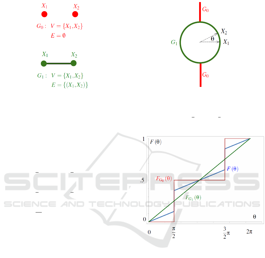
Figure 1: An enumeration of the Gaussian graphical mod-
els for the bivariate normal distribution. Graph G
0
corre-
sponds to independent normal variables x
1
and x
2
. Graph
G
1
corresponds to the general case where covariance struc-
ture between normal variables x
1
and x
2
is unrestricted.
Equation 3 defines the “uniform prior” for these two graphs
(Giudici and Green, 1999, § 1.2).
Figure 2: Geometric interpretation of the relative alignment
parameter θ for a bivariate standard normal distribution.
σ
1 2
= E (x
1
· x
2
) = E(|x
1
||x
2
|cos(θ)) = cos (θ).
Equation 4 permits θ =
1
2
π and θ =
3
2
π for G
0
;
Equation 5 permits 0 ≤ θ ≤ 2π for G
1
.
The unconditional prior p(θ) illustrated in Fig-
ure 3 is:
p(θ) = p (θ|G
0
) p (G
0
) + p(θ|G
1
) p (G
1
) (6)
=
1
4
if θ =
1
2
π ,
1
4
if θ =
3
2
π ,
1
4π
dθ otherwise.
(7)
We find priors assigning point mass to continuous pa-
rameters objectionable. With that caveat, the remain-
der of the Bayesian GGM model comparison frame-
work proceeds as follows. The evidence P(X |g) for
structure g is:
P(X|g) =
Z
P(X|θ,g)P (θ|g)dθ , (8)
and the probability of graph g given the data X is:
P(g|X) ∝ P(X|g)P(g) . (9)
We like the Bayesian model selection approach in
MacKay (1992) and the more recent computational
advances in Skilling (2004). However, Bayesian
GGM approach never gives the process a fair shake.
The number of graphs is 2
(p−1)p/2
. Assuming a uni-
form prior over the graphs as proposed in Giudici and
Green (1999),
2
(p−1)p/2
− 1
/2
(p−1)p/2
≈ 1 of the prior mass is as-
signed to specified points for the continuous natural
parameters. Any finite set of points should collec-
tively have zero probability with a “reasonable prior”
Figure 3: A “uniform prior” on the graphs in Figure 1 re-
sults in a “degenerate prior” for θ in Figure 2. p(θ|G
0
)
defined in Equation 4, p(θ|G
1
) defined in Equation 5, and
p(θ) defined in Equation 7. Cumulative probability F (φ) =
Z
φ
0
p(θ)dθ.
(for continuous parameters). We view the Bayesian
GGM priors as so inequitable, only an unrealistic
number of observations n → ∞ will mitigate its effect.
4 RELATED ARGUMENTS
The beauty of Bayesian methods is the ability to gen-
erate reasonable inference from “complex” models
with limited data. Andrew Gelman’s blog provides
many insightful comments and references relevant to
The Wrong Tool for Inference - A Critical View of Gaussian Graphical Models
473

the issues we wrestle with in this paper. A number
of lively, good natured debates on the blog encour-
aged the use of “complex”
2
models. We view sparse
GGMs as a misguided attempt to maintain parsimony
and simplicity. The following comments encouraged
us to question the wisdom of pursuing simplicity or
parsimony with GGMs.
Gelman (2004) identifies (Neal, 1996, pp. 103-
104) as a favorite quote:
Sometimes a simple model may outperform a
more complex model, at least when the train-
ing data is limited. Nevertheless, I believe
that deliberately limiting the complexity of the
model is not fruitful when the problem is evi-
dently complex. Instead, if a simple model is
found that outperforms some particular com-
plex model, the appropriate response is to de-
fine a different complex model that captures
whatever aspect of the problem led to the sim-
ple model performing well.
A comment that appears specifically related to our
discomfort with uniform priors over the graphs and
point mass distributions for continuous model param-
eters appears in Gelman (2011):
The Occam applications I don’t like are the
discrete versions such as advocated by Adrian
Raftery and others, in which some version of
Bayesian calculation is used to get results say-
ing that the posterior probability is 60%, say,
that a certain coefficient in a model is exactly
zero. I’d rather keep the term in the model and
just shrink it continuously toward zero.
Gelman (2013) nicely clarified that over-fitting is
not attributable to flexibility alone (i.e. the complete
graph in GGMs):
Overfitting comes from a model being flexible
and unregularized. Making a model inflexible
is a very crude form of regularization. Often
we can do better.
5 PREFERABLE METHODS
5.1 Option One
For high dimensional Gaussian inference we first
suggest a full Bayesian implementation as outlined
in (Dempster, 1969, Ch. 15.3) and its equivalent
(Hoff, 2009, Ch. 7). Starting with a prior for the
2
We put “complex” in quotes because its not clear that high
dimensionality alone equates to complexity; and, a log
quadratic density certainly is not that “complex.”
mean p (µ) ∼ N (µ
0
,Λ
0
) and the variance p(Σ) ∼
inverse-Wishart
ν
0
,S
−1
0
, the conditional posterior
distributions are:
p(µ|x
1
,... , x
n
,Σ) ∼ N(µ
n
,Λ
n
) (10)
p(Σ|x
1
,... , x
n
,µ) ∼ inverse-Wishart
ν
n
,S
−1
n
(11)
where
Λ
n
=
Λ
−1
0
+ nΣ
−1
−1
(12)
µ
n
= Λ
n
Λ
−1
0
µ
0
+ nΣ
−1
¯
x
(13)
ν
n
= ν
0
+ n (14)
S
n
= S
0
+ S
µ
(15)
S
µ
=
n
∑
i=1
(x
i
− µ)(x
i
− µ)
T
(16)
The joint posterior p (µ, Σ|x
1
,... , x
n
) is available from
a Gibbs sampler using these conditional distributions
Equation 10 and Equation 11.
5.1.1 Implementation Considerations
Transforming the sampling problem to a set of in-
dependent variables, (Dempster, 1969, Thrm. 12.4.1)
quoted in subsubsection 2.2.2 facilitates straight for-
ward parallel implementation of Equation 10 and
Equation 11 in a Gibbs sampler. Sherman-Morrison-
WoodburyBindel (2009) will be helpful in computing
S
−1
n
in Equation 11 and Λ
n
in Equation 12, treating
the n p samples as low n rank updates to the p × p
diagonal matrices S
−1
0
and Λ
0
respectively.
5.2 Option Two
The second alternative where both p and n are very
large would be to use a maximum entropy algorithm.
Assuming streaming data, one would define a set of
domain specific marginals of interest – for example,
the filters in Zhu (1996) and the gene regulatory net-
work modules in Celik et al. (2014). We would then
implement a maximum entropy algorithm beginning
with the identity matrix and use the framework of
Bretthorst (2012) to determine a posterior distribu-
tion for both the number of constraints and the range
of Lagrange multiplier values defining the synthe-
sized distribution. Bretthorst (2012) nicely demon-
strates Bayesian inference of the appropriate number
of marginal constraints and inference as to the distri-
bution of Lagrange multipliers enforcing a particular
constraint. A final consideration in a dynamic envi-
ronment would be a method to gracefully forget past
observations – perhaps randomly removing one ob-
servation at each iteration to keep a recent weighted
constant size sample; or perhaps weighting the obser-
vations vectors directly for a finite horizon.
ICPRAM 2018 - 7th International Conference on Pattern Recognition Applications and Methods
474

6 CONCLUSION
The dominant discrete theme of GGM obscures
the continuous convex properties of the multivariate
Gaussian distribution. Restricting inference to a par-
ticular graphical model obstructs accumulation of in-
formation describing the underlying distribution. For
Bayesian GGMs, uniform priors over the graphs re-
sults in extremely concentrated probability mass in
the natural parameters.
We support the use of GGMs for interpretation
and communication of approximate inference results
from multivariate Gaussian distributions. We strongly
discourage the use of GGMs directly for multivariate
Gaussian inference.
REFERENCES
Banerjee, O., Ghaoui, L. E., d’Aspremont, A., and Nat-
soulis, G. (2006). Convex optimization techniques for
fitting sparse gaussian graphical models. In Proceed-
ings of the 23rd international conference on Machine
learning, pages 89–96. ACM.
Bindel, D. (2009). Sherman-Morrison-Woodbury. Matrix
Computations (CS 6210), Cornell University lecture.
Bretthorst, G. (2012). The maximum entropy method of
moments and Bayesian probability theory. In 32nd
International Workshop on Bayesian Inference and
Maximum Entropy Methods in Science and Engineer-
ing, Carching, Germany, pages 3–15.
Celik, S., Logsdon, B., and Lee, S. (2014). Efficient di-
mensionality reduction for high-dimensional network
estimation. In Proceedings of the 31st International
Conference on Machine Learning (ICML-14), pages
1953–1961.
Dahl, J., Roychowdhury, V., and Vandenberghe, L. (2005).
Maximum likelihood estimation of Gaussian graphi-
cal models: numerical implementation and topology
selection. Technical report, Department of Electrical
Engineering, University of California, Los Angeles.
Dempster, A. (1969). Elements of continuous multivariate
analysis. Addison-Wesley.
Dempster, A. (1972). Covariance selection. Biometrics,
pages 157–175.
Dobra, A. and West, M. (2004). Bayesian covariance selec-
tion. Duke Statistics Discussion Papers, 23.
Fan, J., Feng, Y., and Wu, Y. (2009). Network exploration
via the adaptive lasso and scad penalties. The Annals
of Applied Statistics, 3(2):521.
Friedman, J., Hastie, T., and Tibshirani, R. (2008). Sparse
inverse covariance estimation with the graphical lasso.
Biostatistics, 9(3):432–441.
Gelman, A. (2004). Against parsimony. [Online; accessed
15-April-2015].
Gelman, A. (2011). David MacKay and Occam’s Razor.
[Online; accessed 15-April-2015].
Gelman, A. (2013). Flexibility is good. [Online; accessed
20-May-2015].
Giudici, P. and Green, P. (1999). Decomposable graph-
ical Gaussian model determination. Biometrika,
86(4):785–801.
Gonzalez, J. and Hong, S. (2008). Linear-time in-
verse covariance matrix estimation in Gaussian pro-
cesses. Technical report, Computer Science Depart-
ment, Carnegie Mellon University.
Good, I. J. (1963). Maximum entropy for hypothesis
formulation, especially for multidimensional contin-
gency tables. The Annals of Mathematical Statistics,
34(3):911–934.
Hoff, P. (2009). A first course in Bayesian statistical meth-
ods. Springer Science & Business Media.
Jalobeanu, A. and Guti
´
errez, J. (2007). Inverse covariance
simplification for efficient uncertainty management.
In 27th MaxEnt workshop, AIP Conference Proceed-
ings, Saratoga Springs, NY.
Jones, B., Carvalho, C., Dobra, A., Hans, C., Carter, C., and
West, M. (2005). Experiments in stochastic computa-
tion for high-dimensional graphical models. Statisti-
cal Science, 20(4):388–400.
Knuiman, M. (1978). Covariance selection. Advances in
Applied Probability, pages 123–130.
Lian, H. (2011). Shrinkage tuning parameter selection in
precision matrices estimation. Journal of Statistical
Planning and Inference, 141(8):2839–2848.
MacKay, D. (1992). Bayesian methods for adaptive models.
PhD thesis, California Institute of Technology.
Meinshausen, N. and B
¨
uhlmann, P. (2006). High-
dimensional graphs and variable selection with the
lasso. The Annals of Statistics, pages 1436–1462.
Moghaddam, B., Marlin, B., Khan, M., and Murphy, K.
(2009). Accelerating Bayesian structural inference
for non-decomposable Gaussian graphical models. In
NIPS.
Neal, R. (1996). Bayesian Learning for Neural Networks.
Springer.
Skilling, J. (2004). Nested sampling. Bayesian Inference
and Maximum Entropy Methods in Science and Engi-
neering, 735:395–405.
Tibshirani, R. (1996). Regression shrinkage and selection
via the lasso. Journal of the Royal Statistical Society.
Series B (Methodological), pages 267–288.
Wang, H., Reeson, C., and Carvalho, C. (2011). Dynamic
financial index models: Modeling conditional depen-
dencies via graphs. Bayesian Analysis, 6(4):639–664.
West, M. and Harrison, J. (1997). Bayesian forecasting and
dynamic models. Springer Verlag.
Whittaker, J. (1990). Graphical models in applied multi-
variate statistics. John Wiley & Sons Ltd.
Yuan, M. and Lin, Y. (2007). Model selection and esti-
mation in the Gaussian graphical model. Biometrika,
94(1):19–35.
Zhu, S. (1996). Statistical and computational theories
for image segmentation, texture modeling and object
recognition. PhD thesis, Harvard University.
The Wrong Tool for Inference - A Critical View of Gaussian Graphical Models
475
APPENDIX
Start Stop
(1)
Maximum
Entropy Null
Hypothesis
(2)
Goodness of
Fit Test
(3)
Fail to Reject the
Null Hypothesis
(4)
Reject
Null Hypothesis
(5)
Covariance
Selection
Add constraint
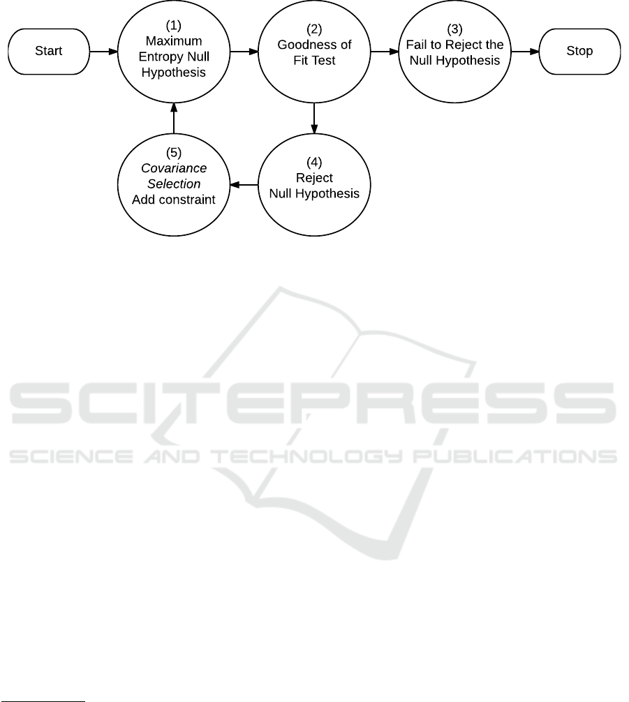
Figure 4: “Covariance Selection” algorithm. “The principle of maximum entropy generates much of statistical mechanics as
a null hypothesis, to be tested by experiment” (Good, 1963, p. 912). The above diagram is the algorithm demonstrated in
Dempster (1972). The diagram accurately describes the algorithm appearing in Zhu (1996).
The Covariance Selection Algorithm
The first sentence of the abstract (Dempster, 1972,
Summary) is misleading:
The covariance structure of a multivariate nor-
mal population can be simplified by setting el-
ements of the inverse of the covariance matrix
to zero.
With respect to the demonstrated algorithm in
(Dempster, 1972, § 3), the widely repeated assertion
that “covariance selection” inserts zeros in a precision
matrix
3
is false. Non-zero entries are placed in a pre-
cision matrix as covariance constraints are added to
a maximum entropy distribution. The matrices gen-
erated are maximally sparse, with non-zeros corre-
sponding to statistically significant structure in the ob-
served data.
The technique demonstrated in (Dempster, 1972,
§ 3) is not about setting elements of the precision ma-
trix (inverse of the covariance matrix) to zero. As
shown in Figure 4, the technique is as follows: 1)
propose a maximum entropy distribution for the “null
hypothesis”; 2) test the “null hypothesis” using ob-
served data; 3) if you “fail to reject the null hypothe-
3
For example, (“setting concentrations (elements of the in-
verse covariance matrix) to zero” Knuiman, 1978); (“spec-
ifies that certain elements in the inverse of the variance ma-
trix are zero” Whittaker, 1990, p. 11); (“by setting to zero
selected elements of the precision matrix” Dobra and West,
2004); (“setting to zero some of the elements of the inverse
covariance matrix” Jalobeanu and Guti
´
errez, 2007); (“set-
ting some elements of the precision matrix to zero” Fan
et al., 2009) (“simplified the matrix structure by setting
some entries to zero.” Lian, 2011)
sis,” STOP; otherwise, 4) “reject the null hypothesis;”
5) “Covariance Selection” – add a covariance con-
straint requiring the proposed distribution match the
observed distribution for the marginal with the worst
discrepancy, this augmented proposal is a new “null
hypothesis,” loop to step 1.
Sparsity in the Precision Matrix
Sparsity is a pervasive topic in papers citing Demp-
ster (1972). It is important to observe that the algo-
rithm directly constructs sparse precision matrices.
The maximum number of zeros in the precision ma-
trix occurs at initialization, when the precision matrix
and the variance matrix for the proposed distribution
are both diagonal. Under duress, as a sequence of
proposed models are rejected by the observed data,
“Covariance Selection” adds non-zeros to the preci-
sion matrix. In Table 1, we provide a sequence of cor-
relation matrices that match each stage of (Dempster,
1972, § 3 Tbl. 1 and system output) exactly and we
provide the corresponding sequence of inverse corre-
lation matrices to clarify the non-zero fill pattern to
show that the maximum entropy algorithm in “Co-
variance Selection” defines sparse precision matrices
by construction.
Replicating the Covariance Selection Example
In Table 1, we are able to fully replicate (Dempster,
1972, § 3 Tbl. 1 and system output) using the algo-
rithm defined in Figure 4 by selecting for inclusion
the pair (i, j) = arg max
(i, j)
|S
i, j
− Σ
Σ
Σ
i, j
| in algorithm step
five “Covariance Selection”.
ICPRAM 2018 - 7th International Conference on Pattern Recognition Applications and Methods
476

Table 1: Using the algorithm in Figure 4 and specifying at each iteration a covariance constraint for the variable pair with
the maximum absolute discrepancy between the observed covariance s
i j
and the synthesized covariance σ
i j
, the column Σ
Σ
Σ
below exactly replicates the output of (Dempster, 1972, § 3). Although more iterations are shown in Dempster (1972) and
below, Dempster suggests stopping the algorithm after stage 5 based upon a statistical significance test. We provide for review
the precision matrices at each stage. Note in the “Covariance Selection” algorithm only one symmetric pair of non-zeros (in
bold) enters the precision matrix Σ
Σ
Σ
−1
at each iteration. The algorithm of Dempster (1972) is widely misrepresented as “setting
elements of the precision matrix to zero.” Clearly, zeros reside in the precision matrix Σ
Σ
Σ
−1
from initialization, dropping out
as constraints are imposed.
Σ
Σ
Σ
−1
Σ
Σ
Σ
0
1.000000
1.000000
1.000000
1.000000
1.000000
1.000000
1.000000
1.000000
1.000000
1.000000
1.000000
1.000000
1
1.000000
1.000000
1.000000
1.279033 0.597405
0.597405 1.279033
1.000000
1.000000
1.000000
1.000000
1.000000 -0.467075
-0.467075 1.000000
1.000000
2
1.273150 0.589712
1.000000
1.000000
1.279033 0.597405
0.589712 0.597405 1.552183
1.000000
1.000000 0.216345 -0.463192
1.000000
1.000000
0.216345 1.000000 -0.467075
-0.463192 -0.467075 1.000000
1.000000
3
1.459781 -0.470598 0.589712
-0.470598 1.186631
1.000000
1.279033 0.597405
0.589712 0.597405 1.552183
1.000000
1.000000 0.396583 0.216345 -0.463192
0.396583 1.000000 0.085799 -0.183694
1.000000
0.216345 0.085799 1.000000 -0.467075
-0.463192 -0.183694 -0.467075 1.000000
1.000000
4
1.617232 -0.470598 -0.426898 0.589712
-0.470598 1.186631
-0.426898 1.157451
1.279033 0.597405
0.589712 0.597405 1.552183
1.000000
1.000000 0.396583 0.368826 0.216345 -0.463192
0.396583 1.000000 0.146270 0.085799 -0.183694
0.368826 0.146270 1.000000 0.079794 -0.170837
0.216345 0.085799 0.079794 1.000000 -0.467075
-0.463192 -0.183694 -0.170837 -0.467075 1.000000
1.000000
5
1.617232 -0.470598 -0.426898 0.589712
-0.470598 1.186631
-0.426898 1.157451
1.279033 0.597405
0.589712 0.597405 1.706470 0.422009
0.422009 1.154287
1.000000 0.396583 0.368826 0.216345 -0.463192 0.169344
0.396583 1.000000 0.146270 0.085799 -0.183694 0.067159
0.368826 0.146270 1.000000 0.079794 -0.170837 0.062458
0.216345 0.085799 0.079794 1.000000 -0.467075 0.170763
-0.463192 -0.183694 -0.170837 -0.467075 1.000000 -0.365602
0.169344 0.067159 0.062458 0.170763 -0.365602 1.000000
The Wrong Tool for Inference - A Critical View of Gaussian Graphical Models
477
