
Performance Evaluation and Enhancement of Biclustering Algorithms
Jeffrey Dale
1
, America Nishimoto
1
and Tayo Obafemi-Ajayi
2
1
Department of Computer Science, Missouri State University, Springfield, MO, U.S.A.
2
Engineering Program, Missouri State University, Springfield, MO, U.S.A.
Keywords:
Biclustering, Evaluation, Gene Expression Pattern Recognition, Validation Measures.
Abstract:
In gene expression data analysis, biclustering has proven to be an effective method of finding local patterns
among subsets of genes and conditions. The task of evaluating the quality of a bicluster when ground truth
is not known is challenging. In this analysis, we empirically evaluate and compare the performance of eight
popular biclustering algorithms across 119 synthetic datasets that span a wide range of possible bicluster struc-
tures and patterns. We also present a method of enhancing performance (relevance score) of the biclustering
algorithms to increase confidence in the significance of the biclusters returned based on four internal validation
measures. The experimental results demonstrate that the Average Spearman’s Rho evaluation measure is the
most effective criteria to improve bicluster relevance with the proposed performance enhancement method,
while maintaining a relatively low loss in recovery scores.
1 INTRODUCTION
Biclustering is an effective unsupervised learning tool
for discovering patterns of co-regulated/co-expressed
genes across a subset of samples in gene expression
data analysis (Madeira and Oliveira, 2004; Pontes
et al., 2015a). As the name implies, clustering is
performed simultaneously on both the row and col-
umn dimensions to discover biclusters, which are de-
fined as submatrices in which the group of rows be-
have similarly across the subset of columns contained
in the submatrix. Biclustering is a special case of
pattern-based clustering algorithms (Kriegel et al.,
2009).
In traditional clustering methods, the objective is
to subdivide the entire data matrix into subgroups, or
clusters, which consist of rows (examples) that ex-
hibit more homogeneous patterns across all columns
(features). In biclustering, these homogeneous sub-
groups, or biclusters, do not necessarily span all the
columns. This makes biclustering useful for identi-
fying possible relevant subspaces in the data. There
are two underlying assumptions in biclustering: (i)
the presence of irrelevant features, or of correlations
among subsets of features, may significantly bias
the representation of clusters in the full-dimensional
space. By relaxing the constraint of global fea-
ture space, we could discover more meaningful sub-
groups; and (ii) different subsets of features may be
relevant for different clusters which implies that ob-
jects cluster in subspaces of the data, rather than
across an entire dimension.
In gene expression data analysis, such a problem
formulation is particularly useful because according
to the general understanding of cellular processes,
only a subset of genes is involved with a specific cel-
lular process, which becomes active only under some
experimental conditions (Xu and Wunsch II, 2011).
Usually, the expression levels of many genes are mea-
sured across a relatively small set of conditions or
samples, and the obtained gene expression data are
organized as a data matrix with rows corresponding to
genes and columns corresponding to samples or con-
ditions. However, such a practice is inherently limited
due to the existence of many uncorrelated genes with
respect to sample or condition clustering, or many
unrelated samples or conditions with respect to gene
clustering. Biclustering offers a solution to such prob-
lems by performing simultaneous clustering on both
dimensions as well as automatically integrating fea-
ture selection with clustering without any prior infor-
mation, so that the relations of clusters of genes (gen-
erally, features) and clusters of samples or conditions
(data objects) are established.
Note that the usefulness of biclustering methods
in discovering local patterns that exist among a sub-
set of rows and columns are also applicable to do-
mains beyond the context of gene expression data
202
Dale, J., Nishimoto, A. and Obafemi-Ajayi, T.
Performance Evaluation and Enhancement of Biclustering Algorithms.
DOI: 10.5220/0006662502020213
In Proceedings of the 7th International Conference on Pattern Recognition Applications and Methods (ICPRAM 2018), pages 202-213
ISBN: 978-989-758-276-9
Copyright © 2018 by SCITEPRESS – Science and Technology Publications, Lda. All rights reserved

analysis such analysis of voting data (Hartigan, 1972)
or more recently, collaborative filtering recommenda-
tion systems (Elnabarawy et al., 2016). In the past
two decades, there has been an influx of multiple bi-
clustering algorithms proposed, as reviewed in (Preli
´
c
et al., 2006; Eren et al., 2012; Oghabian et al., 2014;
Pontes et al., 2015a; Roy et al., 2016). A recent re-
view by Pontes et al. (Pontes et al., 2015a) classifies
30 different biclustering algorithms (which is still not
an exhaustive list of all methods proposed in litera-
ture) by their inherent method of determining optimal
biclusters. It separated the algorithms into two main
categories: those based on evaluation measures vs.
those non metric-based. Given that biclustering is an
unsupervised machine learning technique, a key issue
is how to evaluate/rank the goodness of the biclusters
returned by varied algorithms, especially in the situ-
ations where the algorithm return a large number of
biclusters. This task becomes particularly challeng-
ing in absence of ground truth.
The development of effective heuristic and suit-
able evaluation measures is of particular interest to the
biclustering research community (Cheng and Church,
2000; Pontes et al., 2007; Mukhopadhyay et al., 2009;
Ayadi et al., 2009; Pontes et al., 2010). These mea-
sures are based on inherent assumptions about pos-
sible bicluster patterns for gene expression data such
as shifting, scaling or a combination of both. Sev-
eral evaluation measures have been proposed for bi-
clustering algorithms (Pontes et al., 2015b). These
evaluation measures, also referred to as quality mea-
sures, attempt to quantify the goodness of the biclus-
ters. They can be regarded as internal validation mea-
sures as they are evaluating the biclusters based on
certain desired properties of possible patterns (shift-
ing, scaling, and combined). Pontes et al. in (Pontes
et al., 2015b) conducted a comparison analysis of 14
measures known in literature to assess their ability to
identify optimal biclusters based on shifting, scaling
or combined patterns. Their work identified two of
these measures, average Spearman’s rho (ASR) and
transposed virtual error (VE
T
) as been proficient in
identifying all three types of biclusters.
In this work, we conduct a comparative empir-
ical analysis of the performance of a subset of the
30 algorithms recently identified in (Pontes et al.,
2015a), along with two improved algorithms that
were not included in the review, using a state of the
art benchmark synthetic dataset (Wang et al., 2016).
We propose an enhancement framework based on ap-
plication of two best-performing validation measures
(ASR and VE
T
) to enhance the performance of bi-
clustering methods specifically in terms of identify-
ing the optimal set of relevant biclusters returned by
the algorithms. In addition, we present a compar-
ative performance analysis of the proposed method
using two other commonly used measures: mean
squared residue (MSR) and scaling mean squared
residue (SMSR). We also apply a statistical measure
(Friedman’s test statistic (Conover and Iman, 1981))
to quantify the significance of the improvements ob-
tained. The objective of this study is to provide em-
pirical evidence that can guide practical applications
of biclustering methods along with these measures in
discovering significant and relevant biclusters. The
remainder of this paper is organized as follows. In
section 2, we present an overview of the algorithms
analyzed in this paper. Section 3 presents a descrip-
tion of the performance evaluation framework utilized
in this paper. The experimental results obtained is il-
lustrated and discussed in section 4 while the conclu-
sion is drawn in section 5.
2 BACKGROUND
2.1 Motivation
Our overall goal in this paper is twofold. The first is
to evaluate empirically the performance of eight com-
monly used biclustering algorithms using benchmark
synthetic dataset that differ from previous surveys to
provide an insight into the overall performance of the
algorithms and an understanding of what types of ap-
plications it’s best suited for. Secondly, we are inter-
ested in improving the overall performance of these
algorithms using evaluation measures that have been
proposed in literature. In the context of this work,
an algorithm performs well if majority of the biclus-
ters returned by the method are relevant and if it dis-
covers (or retrieves) majority of the actual biclusters
present in the data. We formally quantify perfor-
mance based on relevance and recovery scores, as de-
fined in section 3.1. Our hypothesis is that ASR and
VE
T
will result in the most significant improvement
given that they have been demonstrated to success-
fully identify biclusters of shifting, scaling and com-
bined patterns (known pattern concepts for gene ex-
pression data (Pontes et al., 2010)). We compare their
effect on the enhancement of these algorithms to MSR
and SMSR which have been demonstrated in litera-
ture as been effective internal validation measures for
only one class of bicluster patters, shifting and scaling
respectively.
It is commonly known that finding biclusters is an
NP-hard problem (Pontes et al., 2015b). Each algo-
rithm usually has its own internal method of guiding
its search for the optimal set of biclusters. Some are
Performance Evaluation and Enhancement of Biclustering Algorithms
203

based on using a heuristic search guided by evalua-
tion measures i.e. metric-based, of which MSR is
the most commonly used, while others are non-metric
based (Pontes et al., 2015a). Given that our goal is to
improve the outcome of these algorithms using evalu-
ation measures, we evaluate algorithms that belong to
both categories and analyze the effect of our proposed
method.
To ensure an unbiased systematic evaluation of
these methods, we selected algorithms that had freely
available implementations and have been readily
cited/used among the biclustering community. Two
of the methods described in this work were an ex-
tension/improvement of a prior method reviewed
among the 30 biclustering algorithms in (Pontes et al.,
2015a). In this work, we focused on the most re-
cent improved method (as in the case of UniBic and
BicPAMS described below). Table 1 presents an
overview of the 8 algorithms empirically evaluated
and analyzed in this work including the implemen-
tation source. They include both metric-based and
non-metric based approaches and span two decades.
To provide a context for the comparative analysis pre-
sented in this paper, we briefly describe each biclus-
tering algorithm in a chronological order.
2.2 Review of Biclustering Algorithms
Cheng and Church (CC)
The Cheng and Church algorithm (Cheng and
Church, 2000) was the first application of biclustering
to finding local similarity patterns in gene expression
data. CC is a deterministic greedy algorithm that finds
biclusters by minimizing the Mean Squared Residue
(MSR) score of a discovered submatrix. MSR is
an evaluation measure that is a measure of bicluster
homogeneity, as defined in the next section. As a
heuristic-based method, it outputs a desired number
of biclusters k based on user defined parameters k and
δ, which is the maximum acceptable MSR score.
Iterative Signature Algorithm (ISA)
The iterative signature algorithm (Bergmann et al.,
2003) is a non-deterministic method that discov-
ers biclusters even in the presence of noise and
overlapping biclusters. It defines the biclusters as
transcription modules (TM): a set of co-regulated
genes (rows) with relevant experimental conditions
(columns). Starting from a set of randomly selected
genes (or conditions), it iteratively refines the genes
and conditions until they match the definition of TM.
In the context of this work, we evaluate ISA as a non-
heuristic based method (Pontes et al., 2015a) though
in some others reviews (Preli
´
c et al., 2006; Eren
et al., 2012), it has been evaluated as a heuristic based
method due to its iterative greedy search approach.
Order-Preserving Submatrices
Algorithm (OPSM)
The Order-Preserving Submatrices Algorithm (Ben-
Dor et al., 2003) is a deterministic method for finding
biclusters that are defined as order-preserving subma-
trices i.e. a set of rows and columns in the data matrix
in which all the values in the rows for the given set of
columns are strictly increasing (or similarly ordered
in the relaxed case). Using a probabilistic model de-
scribing biclusters hidden in otherwise random ma-
trices and statistical strategies, OPSM algorithm can
efficiently find multiple, potentially overlapping bi-
clusters.
FLexible Overlapped biClustering
(FLOC)
The Flexible Overlapped Biclustering algorithm
(Yang et al., 2005) is a stochastic iterative based
method for finding biclusters, particularly overlap-
ping ones using a probabilistic model. It is an
evaluation-based approach that assesses the quality of
the biclusters using the mean residue function, similar
to the CC algorithm. It consists of two steps. In the
first step, crude initial biclusters are constructed on a
probabilistic basis. The second step centers around
iteratively refining these biclusters. This process in-
volves greedily removing rows or columns from the
bicluster in an effort to reduce the mean squared
residue score of the bicluster.
Factor Analysis for Bicluster Acquisition
(FABIA)
The Factor Analysis for Bicluster Acquisition method
(Hochreiter et al., 2010) is a generative multiplicative
model for discovering biclusters in expression data
by assuming a non-Gaussian signal distributions with
heavy tails. (This method was not included in the re-
view presented in (Pontes et al., 2015a).) In FABIA, a
bicluster is modeled as an outer product of two sparse
vectors. It is a fuzzy like clustering method that re-
turns probability of memberships. However, it can be
set to return crisp biclusters by setting user-defined
threshold parameters.
ICPRAM 2018 - 7th International Conference on Pattern Recognition Applications and Methods
204

Table 1: Biclustering Algorithm Summary.
Algorithm (Year) Algorithm Type
Deterministic /
Implementation Source
Metric based
CC (2000) Greedy Search Yes / Yes (MSR) Python (Eren, 2013)
ISA (2003) Linear Algebra Yes / No R package isa2 (Cs
´
ardi et al., 2010)
OPSM (2003) Optimal Reordering Yes / No BicAT (Barkow et al., 2006)
FLOC (2005) Stochastic Greedy Search No / Yes (MSR) R Package BicARE (Gestraud, 2008)
FABIA (2010) Generative Biclustering No / No Bioconductor fabia (Hochreiter et al., 2010)
PPM
3
(2015) Probabilistic No / No Java (Chekouo and Murua, 2015)
UniBic
2
(2016) Graph-Based No / No C (Wang et al., 2016)
4
BicPAMS
1
(2017) Pattern-based No / No bicpams.com (Henriques et al., 2017)
1
Most recent pattern mining approach.
2
Improvement on the QUBIC algorithm.
3
Extension of Bayesian Biclustering Model.
4
sourceforge.net/projects/unibic/
Penalized Plaid Model (PPM)
The Penalized Plaid Model biclustering technique
(Chekouo and Murua, 2015) models biclusters using
a Bayesian framework. It is a modified extended ver-
sion of the Bayesian plaid model. The PPM method
fully accounts for a general overlapping structure,
which differs from other models that account for only
one dimensional overlapping such as in the Bayesian
Biclustering Model (Gu and Liu, 2008). Instead of us-
ing the sequential algorithm defined in (Zhang, 2010),
the parameters in the Penalized Plaid model are found
all at once by a dedicated Markov chain Monte Carlo
sampler. It is a non-heuristic based approach.
UniBic
UniBic is an extension/improvement of the graph-
based biclustering method: QUBIC (Li et al., 2009).
In this work, we evaluate UniBic, which was not re-
viewed in (Pontes et al., 2015a) since it’s an improved
algorithm of QUBIC that was included in (Pontes
et al., 2015a). In QUBIC, the input data matrix is
initially transformed to a discrete integer rank matrix
prior to subsequent operations. A graph G is con-
structed based on this matrix in which nodes repre-
sent the rows (genes) and the edge weights are num-
ber of corresponding conditions (columns) between
two genes (rows). The biclustering problem is trans-
lated to finding heavy subgraphs in G.
UniBic (Wang et al., 2016) is very similar to
QUBIC with the exception of edge weight calcu-
lation. UniBic applies the longest common subse-
quence (LCS) algorithm to translate the input data
matrix to a rank matrix in which the rows are dis-
cretized as rank vectors. The n
th
smallest value in
each row is replaced with the integer n, with priority
in ties given to the leftmost value. Edge weight in the
graph is calculated as the magnitude of the maximal
LCS between nodes. UniBic demonstrates a strong
resilience to noise and can detect biclusters of both
shifting and scaling patterns.
Biclustering based on PAttern Mining
Software (BicPAMS)
BicPAMS (Henriques et al., 2017) is an aggregate of
state-of-the-art pattern mining approaches to the bi-
clustering problem. BicPAMS is the most recent pat-
tern mining algorithms, an improved version of prior
pattern mining biclustering algorithms since the ini-
tial publication of BicPAM (Henriques and Madeira,
2014a). Other prior versions of pattern-mining biclus-
tering algorithms that it extends include BicSPAM
(Henriques and Madeira, 2014b) (reviewed in (Pontes
et al., 2015a)), BiP (Henriques and Madeira, 2015),
and BicNET (Henriques and Madeira, 2016). Bic-
PAMS is a highly parametrized algorithm includ-
ing parameters relating to coherence of biclusters,
structure of biclusters, quality of biclusters, and ef-
ficiency of the program. BicPAMS was not reviewed
in (Pontes et al., 2015a). It is a non-heuristic based
algorithm.
3 METHODS
3.1 Evaluation Framework
To effectively evaluate the biclustering algorithms,
we utilize the benchmark synthetic data introduced
in (Wang et al., 2016) and generated with the
BiBench framework (Eren et al., 2012). The ad-
vantage of utilizing synthetic data in evaluation of
algorithm performance is that there is readily avail-
able ground-truth. However, there is always the con-
cern of whether the synthetic data generation cap-
tures the complexity of real applications. The bench-
mark data consist of 6 groups of square bicluster
Performance Evaluation and Enhancement of Biclustering Algorithms
205

structures (trend-preserving, column-constant, row-
constant, shift-scale (combined), shift, scale) as well
as 3 overlapping datasets and 3 narrow datasets: a to-
tal of 119 datasets. Square biclusters have the same
number of genes and conditions in each bicluster
while overlapping biclusters are biclusters that share
one or more genes or conditions. Narrow biclusters
contain many more genes than conditions. A com-
prehensive description of these bicluster types is pre-
sented in (Mukhopadhyay et al., 2010).
Given a bicluster B , let I denote a set of row vec-
tors in B and J, the corresponding set of column vec-
tors. Then, the element in the i
th
and j
th
column of B
is denoted by B
i j
. We index specific gene vectors or
condition vectors using capital letters. For example,
the gene corresponding to the i
th
row of B across all
conditions is denoted B
iJ
, while the condition corre-
sponding to the j
th
column of B across all genes is
denoted B
I j
.
To evaluate the performance of the algorithms,
we utilize the recovery and relevance scores, derived
from match score (Preli
´
c et al., 2006). Match Score
(MS) between two sets of biclusters S
1
and S
2
is de-
fined as:
MS (S
1
, S
2
) =
1
|S
1
|
∑
B
1
∈S
1
max
B
2
∈S
2
|B
1
∩ B
2
|
|B
1
∪ B
2
|
(1)
which reflects the average of the maximum similarity
for all biclusters B
1
in S
1
with respect to the biclusters
B
2
in S
2
. The intersection of two biclusters B
1
∈ S
1
and B
2
∈ S
2
denotes the set of rows common to both
B
1
and B
2
. Similarly, the union of two biclusters is
the set of rows that exist in either B
1
or B
2
or both.
The match score takes on values between 0 and 1,
inclusive. In the case that no rows of any bicluster
in S
1
are found in any bicluster in S
2
, |B
1
∩ B
2
| = 0
for all possible B
1
∈ S
1
, B
2
∈ S
2
. Subsequently, MS
= 0 (equation (1). Similarly, if the sets of biclusters
S
1
and S
2
are identical, then both |B
1
∩ B
2
| = |S
1
|
and |B
1
∪ B
2
| = |S
1
|, yielding a match score of one.
The match score is also referred to as similarity score
(Wang et al., 2016).
For a given dataset D, let S(A
i
) denote the set of
biclusters returned by applying a specific biclustering
algorithm A
i
on D, while G denotes the correspond-
ing set of known ground truth biclusters for D. The
relevance score, MS(S, G), is a measure of the ex-
tent to which the generated biclusters S(A
i
) are sim-
ilar to the ground truth biclusters in the gene (row)
dimension. The recovery score, given by MS(G, S),
quantifies the proportion of the subset of G that were
retrieved by A
i
. A high relevance score implies that
a large percentage of the biclusters discovered by the
algorithm are significant, while a high recovery score
indicates that a large percentage of the actual ground
truth biclusters are very similar to the ones returned
by the algorithm.
3.2 Internal Validation Measures
Relevance and recovery scores are both external
validation measures, as the computation is dependent
on prior knowledge of ground truth data. Internal
validation measures provide a means of evaluating
quality of biclusters obtained without the knowledge
of ground truth; which is very useful for real datasets
for which ground truth is unknown. In this section,
We formally describe the two evaluation measures
that are used in our performance enhancement
method: ASR and VE
T
. We also discuss two other
common internal validation measures that we utilize
for comparison analysis: MSR and SMSR.
Average Spearman’s Rho. The Average Spearman’s
Rho (ASR) (Ayadi et al., 2009) measure is an adapta-
tion of the Spearman’s Rho (Lehmann and D’abrera,
1975) correlation coefficient to assess bicluster qual-
ity. Spearman’s Rho is defined as
ρ(x, y) = 1 −
6
m(m
2
− 1)
m
∑
k=1
(r (x
k
) − r (y
k
))
2
(2)
for two vectors x and y of equal length m, where r(x
k
)
and r(y
k
) are the ranks of x
k
and y
k
, respectively. Let
ρ
gene
=
∑
i∈I
∑
j∈I, j>i
ρ(i, j)
|I| · (|I|− 1)
(3)
ρ
condition
=
∑
i∈J
∑
j∈J, j>i
ρ(i, j)
|J| · (|J| − 1)
(4)
ASR is defined as
ASR(B) = 2 · max
{
ρ
gene
, ρ
condition
}
(5)
The ASR’s value is in the range [−1, 1], where both
−1 and 1 represent a perfect trend-preserving biclus-
ter. ASR is one of the few bicluster quality measures
that can detect both shifting and scaling patterns of
biclusters, as well as shift-scale (combined pattern)
biclusters (Pontes et al., 2015b).
Transposed Virtual Error. Transposed Virtual Er-
ror (VE
T
) (Pontes et al., 2010) is another bicluster
quality measure that correctly identifies shift, scale,
and shift-scale biclusters. Transposed Virtual Error is
an improvement on Virtual Error (VE) (Pontes et al.,
2007), which does not identify shift-scale biclusters.
Both VE and VE
T
required standardized biclus-
ters. A bicluster is standardized by subtracting the
row mean from each element of the bicluster and di-
viding by the row standard deviation, i.e.
ICPRAM 2018 - 7th International Conference on Pattern Recognition Applications and Methods
206

ˆ
B =
B
i j
− µ
iJ
σ
iJ
, i = 1, 2, ..., |I|, j = 1, 2, ..., |J|
(6)
where µ
iJ
is the mean of row i in B and σ
iJ
is the
standard deviation of row i in B.
VE computes a virtual gene ρ, which is a vec-
tor imitating a gene whose entries are column means
across all genes in the bicluster. Explicitly, the stan-
dardized virtual gene is calculated for a standardized
bicluster
ˆ
B as
ˆ
ρ
j
=
1
|I|
|I|
∑
i=1
ˆ
B
i j
, j = 1, 2, ..., |J| (7)
Finally, VE is defined as
V E(B) =
1
|I| · |J|
|I|
∑
i=1
|J|
∑
j=1
|
ˆ
B
i j
−
ˆ
ρ
j
| (8)
To compute VE
T
, transpose the bicluster prior to cal-
culating VE. VE
T
computes a virtual condition ρ and
measures the deviation of conditions in the bicluster
from ρ. The virtual condition ρ is calculated as
ˆ
ρ
i
=
1
|J|
|J|
∑
j=1
ˆ
B
i j
, j = 1, 2, ..., |J| (9)
and VE
T
is calculated as
V E
T
(B) =
1
|I| · |J|
|I|
∑
i=1
|J|
∑
j=1
|
ˆ
B
i j
−
ˆ
ρ
i
| (10)
VE
T
is equal to zero for perfect shifting or scaling
or shift-scale patterns.
Special Cases for VE
T
. Constant rows in expression
data pose an issue when computing VE
T
. When one
or more rows are constant, the standard deviation of
at least one row is zero, and thus the result of equation
(3.2) is undefined.A constant row is highly unlikely
in real data applications, so a standard deviation of
zero should be a non-issue. For the context of this
work with synthetic data, VE
T
is set to one if any
zero-division errors occurred. This does produce
false negatives in the case that a constant row is part
of a constant bicluster.
Mean Squared Residue. The mean squared residue
score (MSR) describes how well a bicluster follows a
shifting pattern (Cheng and Church, 2000). MSR is
defined as
MSR(B) =
1
|I| · |J|
|I|
∑
i=1
|J|
∑
j=1
(b
i j
−b
iJ
−b
I j
+b
IJ
)
2
(11)
where the bicluster B consists of rows I and columns
J. Values b
iJ
and b
I j
denote the mean of the i
th
row and j
th
column, respectively, and b
IJ
denotes the
mean of all entries of the bicluster.
By design, biclusters that follow a perfect shifting
pattern have an MSR score of zero. Larger MSR
scores represent more deviation from a perfect
shifting pattern.
Scaling Mean Squared Residue. The Scaling Mean
Squared Residue (SMSR) is an evaluation measure
for biclusters that detects scaling patterns in biclusters
(Mukhopadhyay et al., 2009). SMSR is very similar
to MSR except that it is suited for biclusters with scal-
ing patterns while MSR is suited for shifting patterns.
SMSR is defined as
SMSR(B ) =
1
|I| · |J|
|I|
∑
i=1
|J|
∑
j=1
(b
iJ
· b
I j
− b
i j
· b
IJ
)
2
b
2
iJ
· b
2
I j
(12)
The SMSR score of a bicluster with a perfect scaling
pattern is zero. Neither MSR nor SMSR perform well
on shift-scale biclusters.
3.3 Enhancement Framework
Gene expression data matrices are usually very large.
It is not uncommon for these matrices to have tens of
thousands of rows (genes) and hundreds of columns
(samples). It is generally unknown how many biclus-
ters will be returned by a biclustering algorithm on
a given dataset. Some biclustering algorithms usu-
ally output a very large set of biclusters (based on al-
gorithm specific stop criterion) while some include a
user specified parameter to define the number of bi-
clusters to generate. A large portion of recent bi-
clustering algorithms use stochastic approaches, and
hence are not deterministic. This means that multi-
ple repetitions of the same experiment with such algo-
rithms do not necessarily yield identical results. Prop-
erties of algorithms analyzed in this paper, such as
determinism vs. non-determinism, are described in
Table 1. It is desirable for the discovered set of bi-
clusters to be a manageable number of highly relevant
since the discovered biclusters require significant hu-
man effort for further evaluation to determine biolog-
ical significance.
In this section, we present a method of improv-
ing the relevance score of any set of biclusters by us-
ing either of these two internal validation measures:
Average Spearman’s Rho and Transposed Virtual Er-
ror. This can be applied to both types of algorithms
i.e. the ones that have a defined stop criterion as
well as the ones that require a user-specified parame-
ter of number of biclusters to generate. The strength
of the proposed framework is that it serves a ”filter” to
help detect highly relevant bicluster among a large set
Performance Evaluation and Enhancement of Biclustering Algorithms
207

of output biclusters. The framework can be applied
using any desired internal validation metric, though
from the results obtained, we recommend using the
best performing ones (VE
T
and ASR). The next step
is to determine an ensemble method for leveraging the
usefulness of both metrics.
The method of improving the relevance of a set of
biclusters S is described as follows:
1. Choose an internal validation measure M and a
number of desired biclusters n, where n < |S|.
2. Compute M(B ) for each bicluster B ∈ S .
3. Order each bicluster in B ∈ S from best to worst
according to M(B).
4. Retain the best n biclusters according to M.
It is important to note that while relevance scores are
improved with our method, recovery scores are nega-
tively impacted. By reducing the number |S|, the ini-
tial size of the output biclusters, the recovery score
will be less than or equal to that of the initial list.
Thus, our goal is to maximize the increase in rele-
vance scores while minimizing the decrease in recov-
ery scores. Ideally, we desire to filter out biclusters
with redundant or insignificant information.
4 EXPERIMENTAL RESULTS
AND ANALYSIS
4.1 Experimental Setup
The eight biclustering algorithms analyzed in this
work were set to their default parameters and con-
ducted using existing implementations (Table 1). To
ensure that the experiments presented in this work are
replicable, the source code is publicly available via
GitHub
1
along with detailed instructions on the spec-
ifications of implementations. For algorithms (CC,
FLOC, and PPM)that required user-specified param-
eter k on the number of biclusters to generate, we set
k = 20. In addition, CC was set to return biclusters
with a maximum MSR score of 0.1. For OPSM, the
number of passed models between iterations used was
10. PPM was implemented using the recommended
parameters of the GPE method (Chekouo and Murua,
2015).
In the computation of ASR, we have to compute
Spearman’s Rho according to equation (2). This re-
quires us calculate the rank of each element in both
vectors x and y. When there are ties in the elements
1
github.com/clslabMSU/Biclustering-Algorithm-
Comparison
of x or y, ranking becomes problematic and subse-
quently results in Spearman’s Rho not being defined.
There are different tie correction methods available to
alleviate this problem (Zar, 1998). The method of tie
correction implemented in this work was to assign all
tied values to the minimum rank.
The experimental results presented are two-fold.
In section 4.2, we present the results of the compar-
ative analysis of the eight algorithms using relevance
and recovery scores on the 119 benchmark datasets
while section 4.3 focuses on empirical evaluation of
the proposed enhancement framework. For the per-
formance enhancement evaluation, the desired num-
ber of biclusters n is set to 3g, where g is the actual
number of biclusters present in the dataset (based on
the ground truth information). Thus, the evaluation
results presented demonstrate the impact on both rel-
evance and recovery scores with a very minimal num-
ber of clusters selected - 3g. In actual practice, n can
be set to the number that the user is comfortable using
for further biological evaluation.
4.2 Performance Evaluation Results
Figure 1 illustrates the results of the performance of
the eight algorithms in terms of relevancy and recov-
ery scores for eight types of biclusters datasets: 6
types of square biclusters (trend-preserving, column-
constant, row-constant, shift-scale (combined), shift,
scale) with each type having 15 associated datasets,
as well as a set of 20 overlapping datasets and a set of
9 narrow datasets.
As can be observed from Figure 1a, OPSM is
the best performing algorithm on narrow biclusters
in terms of both relevance and recovery scores. This
is useful for practical gene expression datasets where
the number of conditions is much less than the num-
ber of genes. For the datasets with overlapping bi-
clusters (Figure 1b), BicPAMS performed the best
in terms of relevance, and UniBic performed best in
terms of recovery. For all the datasets, except for nar-
row, UniBic had very high recovery scores.
Table 2 illustrates the average rank of each algo-
rithm across all 119 synthetic datasets. The rank-
ing results for the performance evaluation results is
contained in the first 4 columns after the algorithm
name column (i.e. before enhancement). The aver-
age rank is calculated by ranking each algorithm’s
performance on each dataset, with 1 being the best
performer and 8 (in this case) being the worst. We
rank the performance using relevance and recovery
scores, ASR, and VE
T
. The average rank of an algo-
rithm is simply the sum of its ranks for each dataset
divided by the number of datasets. The statistical sig-
ICPRAM 2018 - 7th International Conference on Pattern Recognition Applications and Methods
208

0
0.1
0.2
0.3
0.4
0.5
0.6
0.7
0.8
0.9
1
0 0.1 0.2 0.3 0.4 0.5 0.6 0.7 0.8 0.9 1
Recovery
Relevance
Narrow Biclusters
ISA CC OPSM BicPAMS
UniBic FABIA FLOC PPM
(a) Narrow Biclusters
0
0.1
0.2
0.3
0.4
0.5
0.6
0.7
0.8
0.9
1
0 0.1 0.2 0.3 0.4 0.5 0.6 0.7 0.8 0.9 1
Recovery
Relevance
Overlap
ISA CC OPSM BicPAMS
UniBic FABIA FLOC PPM
(b) Overlapping Biclusters
0
0.1
0.2
0.3
0.4
0.5
0.6
0.7
0.8
0.9
1
0 0.1 0.2 0.3 0.4 0.5 0.6 0.7 0.8 0.9 1
Recovery
Relevance
Type 1 Biclusters
ISA CC OPSM BicPAMS
UniBic FABIA FLOC PPM
(c) Square Type 1 (trend-preserving) Biclusters
0
0.1
0.2
0.3
0.4
0.5
0.6
0.7
0.8
0.9
1
0 0.1 0.2 0.3 0.4 0.5 0.6 0.7 0.8 0.9 1
Recovery
Relevance
Type 2 Biclusters
ISA CC OPSM BicPAMS
UniBic FABIA FLOC PPM
(d) Square Type 2 (column-constant) Biclusters
0
0.1
0.2
0.3
0.4
0.5
0.6
0.7
0.8
0.9
1
0 0.1 0.2 0.3 0.4 0.5 0.6 0.7 0.8 0.9 1
Recovery
Relevance
Type 3 Biclusters
ISA CC OPSM BicPAMS
UniBic FABIA FLOC PPM
(e) Square Type 3 (row-constant) Biclusters
0
0.1
0.2
0.3
0.4
0.5
0.6
0.7
0.8
0.9
1
0 0.1 0.2 0.3 0.4 0.5 0.6 0.7 0.8 0.9 1
Recovery
Relevance
Type 4 Biclusters
ISA CC OPSM BicPAMS
UniBic FABIA FLOC PPM
(f) Square Type 4 (shift-scale) Biclusters
0
0.1
0.2
0.3
0.4
0.5
0.6
0.7
0.8
0.9
1
0 0.1 0.2 0.3 0.4 0.5 0.6 0.7 0.8 0.9 1
Recovery
Relevance
Type 5 Biclusters
ISA CC OPSM BicPAMS
UniBic FABIA FLOC PPM
(g) Square Type 5 (shift) Biclusters
0
0.1
0.2
0.3
0.4
0.5
0.6
0.7
0.8
0.9
1
0 0.1 0.2 0.3 0.4 0.5 0.6 0.7 0.8 0.9 1
Recovery
Relevance
Type 6 Biclusters
ISA CC OPSM BicPAMS
UniBic FABIA FLOC PPM
(h) Square Type 6 (scale) Biclusters
Figure 1: Comparisons of recovery and relevance scores across biclustering algorithms on different types of bicluster datasets.
Performance Evaluation and Enhancement of Biclustering Algorithms
209

nificance of these ranks is measured using Friedman
test statistic. The critical value of a chi-square distri-
bution with 7 degrees of freedom is 14.067, so Fried-
man statistics higher than 14.067 are considered sta-
tistically significant. The p-values associated with the
Friedman statistics were all significant: < 0.001.
From Table 2, one can observe that BicPAMS had
the best average rank in terms of relevance score be-
fore performance enhancement, and UniBic had the
best average rank in recovery score by a very large
margin. Similarly, OPSM had the best average rank
according to the ASR value (internal validation mea-
sure) in every dataset, hence an average rank of 1.0.
OPSM also had the best average rank according to
VE
T
, closely followed by FLOC.
4.3 Performance Enhancement Results
UniBic and BicPAMS both tended to have high recov-
ery scores but low relevance scores according to the
experimental results in section 4.2. They also returned
a very large number of clusters as indicated in Table 3
which probably helped their recovery scores but de-
graded the performance in terms of relevance. Fig-
ure 2 demonstrates the effect of the performance en-
hancement (PE) framework on the performance of the
algorithms in terms of relevancy and recovery scores.
For each algorithm, the top n biclusters selected is
set to three times the actual number of ground truth
present in the dataset. The algorithms that benefit the
most from the PE method are those that return a very
large number of biclusters, such as BicPAMS and
UniBic. When these algorithms are applied to real
gene expression datasets, the number of returned bi-
clusters is usually too large to manually examine. By
applying the PE method, results of these algorithms
are much more manageable, and each bicluster exam-
ined is more likely to contain biologically significant
information. According to Table 3, PPM algorithm is
the only algorithm that actually returns less than this
parameter initially i.e. before enhancement. Given
that the returned number of biclusters is less, some
loss in recovery is inevitable however, it is interesting
to observe the effect on the relevance of the results.
Table 3 also demonstrates that, overall, applying
the PE framework using the ASR or VE
T
measure
yields a more significant positive impact on the rel-
evance scores compared to MSR or SMSR measures.
We can observe from Figure 2 that relevance scores
were improved for six of the eight tested algorithms,
with the most dramatic improvement being on the
UniBic algorithm and the ASR quality measure. In
this case, the relevance of the UniBic biclusters were
increased by well over 50%. Naturally, removing bi-
clusters from a set will have a negative impact on the
recovery score of that set. The ASR validation mea-
sure showed the largest increase in relevance scores
among every algorithm except OPSM and FABIA,
thus indicating most superior performance compared
to VE
T
, SMSR and MSR. Table 4 summarizes the ef-
fect of the enhancement framework, based only on the
ASR measure according to the eight different types of
dataset tested.
The last two sets of four columns of Table 2
present the average ranking results of each algo-
rithm after applying the PE framework using the ASR
and VE
T
validation measures, respectively across all
datasets. For both evaluation measures, we observe
that the best performing algorithms are largely the
same as before we performed our enhancement. How-
ever, the average ranks have shifted slightly. Filtering
on the ASR measure has further set BicPAMS apart
from the competition in terms of relevance, lowering
its rank from 2.18 before enhancement to 1.62 after
ASR filtering. UniBic still performs best in terms of
recovery, but by a smaller margin. Filtering by VE
T
has produced less compelling results. The average
ranks for recovery are much closer together than the
ranks before enhancement and the ranks using ASR
filtering, which implies that the ranks of each algo-
rithm across all datasets were inconsistent. This is
reflected in the lower Friedman statistics of VE
T
fil-
tering compared to the Friedman statistics before en-
hancement and with ASR filtering.
For the evaluation (metric)-based methods, CC
and FLOC, which are based on MSR, applying ASR
to select the top n biclusters still improves the rele-
vance scores, even though the original mean number
of clusters returned by these algorithm is 20 which is
close to the mean top n that we select [12, 20]. Ac-
cording to Table 3, though recovery scores were hurt,
the algorithm with the highest recovery score was un-
changed after our enhancement, implying that the per-
centage loss was almost uniform across best perform-
ing algorithms. The PE framework results demon-
strate that the ASR quality measure tended to lead
to a larger increase in relevance scores, while main-
taining a relatively low loss in recovery scores. At
this point, it becomes a trade-off between obtaining
a manageable number of biclusters and losing accu-
racy. On larger datasets for real data applications,
it quickly becomes difficult to inspect the biological
significance of a large number of biclusters. Thus,
the proposed PE framework would be useful for gene
expression data analysis, in determining significance
and relevance of the results.
ICPRAM 2018 - 7th International Conference on Pattern Recognition Applications and Methods
210
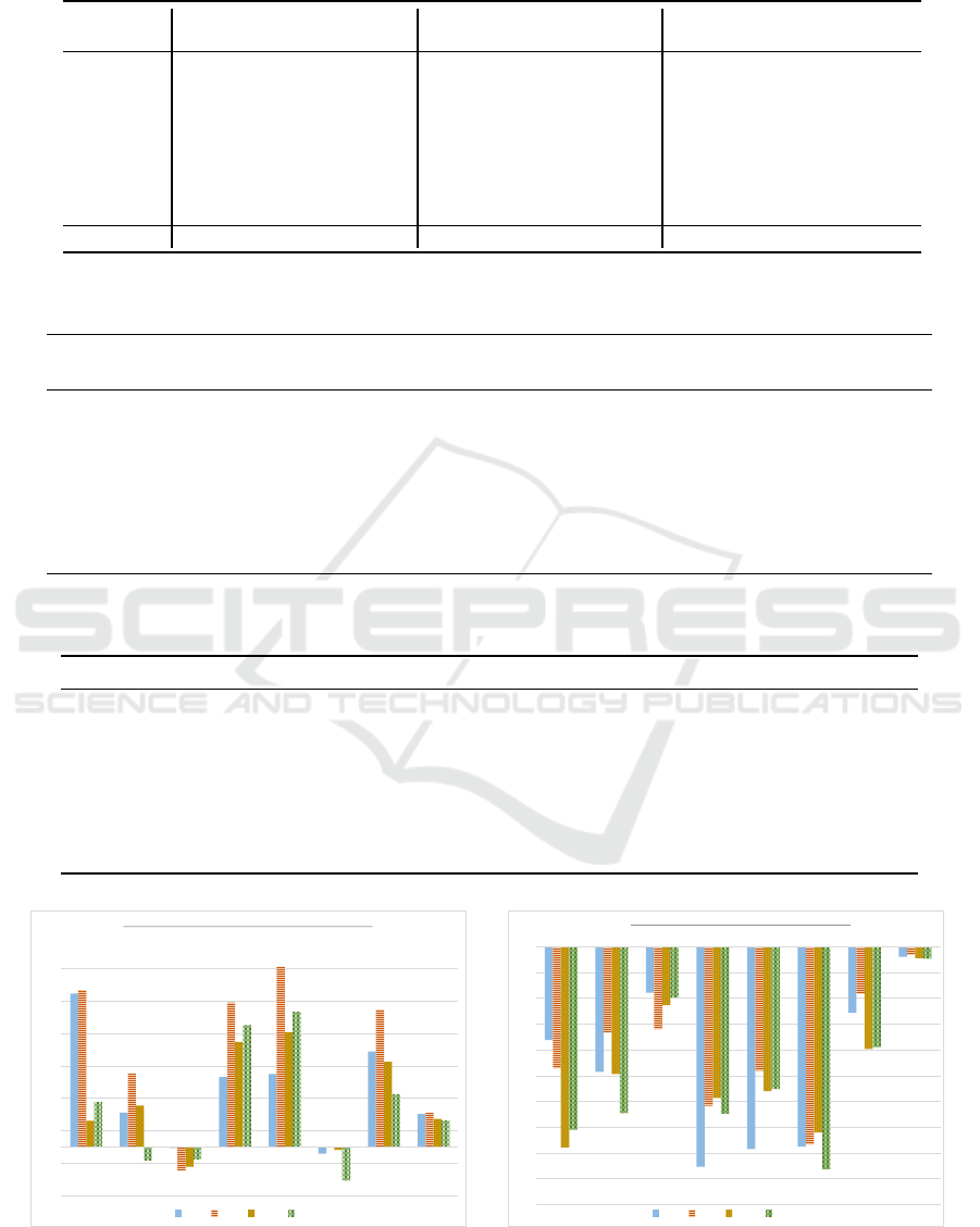
Table 2: Statistical comparison of average ranking of algorithm performance using Friedman test before and after enhancement
method.
Algorithm
Before Enhancement Filtering on ASR Filtering on VE
T
Rel. Rec. ASR VE
T
Rel. Rec. ASR VE
T
Rel. Rec. ASR VE
T
BicPAMS 2.18 2.75 3.39 3.75 1.62 3.62 1.92 2.12 1.67 3.91 2.14 1.62
CC 7.67 7.06 4.43 3.25 7.47 6.86 5.46 3.88 7.55 7.03 5.38 5.25
FABIA 6.10 4.87 7.42 8.00 6.60 5.84 7.48 7.12 6.56 5.69 7.50 8.00
FLOC 4.66 5.12 3.47 1.62 4.28 4.58 4.37 1.25 4.60 4.58 4.09 2.88
ISA 5.04 4.07 6.35 6.62 4.42 3.99 5.26 4.75 4.22 3.39 5.61 5.62
OPSM 2.77 5.42 1.00 1.38 3.73 4.55 1.22 3.50 3.46 4.16 1.03 3.88
PPM 4.09 5.39 5.52 6.00 4.86 4.49 6.46 6.12 4.49 4.22 6.40 7.00
UniBic 3.49 1.32 4.41 5.38 3.03 2.07 3.83 7.25 3.45 3.02 3.85 1.75
Friedman
1
276 290 265 335 289 260 313 390 192 163
?
280 425
Rec.: Recovery Score; Rel.: Relevance Score;
1
P-values for all Friedman tests < 0.001 with the exception of:
?
P-value = 0.004.
Table 3: Mean number of biclusters returned by algorithm.
Biclusters
Range of g
1
PE Exp.
2
Mean No. of biclusters returned by each algorithm.
n = 3g BicPAMS FABIA ISA OPSM PPM UniBic CC FLOC
Narrow 3 9 320 12 65 11 10 92 20 20
overlap 3 9 557 20 26 14 10 53 20 20
Type 1 [3 5] 12 243 20 48 10 10 42 20 20
Type 2 [3 5] 12 746 20 37 10 10 47 20 20
Type 3 [3 5] 12 712 19 46 9 10 61 20 20
Type 4 [3 5] 12 768 19 53 9 10 40 20 20
Type 5 [3 5] 12 353 20 35 10 10 56 20 20
Type 6 [3 5] 12 374 19 53 10 10 43 20 20
1
g: Mean number of biclusters in ground truth data;
2
PE Exp: Performance Enhancement Experiment.
Table 4: Best performing algorithm before and after enhancement (by ASR).
Type of dataset Best relevance before Best recovery before Best relevance after Best recovery after
Narrow Bicluster OPSM OPSM BicPAMS OPSM
Overlap Bicluster BicPAMS UniBic FLOC UniBic
Type 1 Biclusters UniBic UniBic BicPAMS UniBic
Type 2 Biclusters BicPAMS UniBic FLOC UniBic
Type 3 Biclusters FLOC UniBic FLOC UniBic
Type 4 Biclusters UniBic UniBic BicPAMS UniBic
Type 5 Biclusters BicPAMS UniBic BicPAMS UniBic
Type 6 Biclusters UniBic UniBic BicPAMS UniBic
-15%
-5%
5%
15%
25%
35%
45%
55%
ISA CC OPSM BicPAMS UniBic FABIA FLOC PPM
Improvement in Relevance Scores Across Quality Measures
VET ASR MSR SMSR
(a) Improvement in Relevance Scores.
-50%
-45%
-40%
-35%
-30%
-25%
-20%
-15%
-10%
-5%
0%
ISA CC OPSM BicPAMS UniBic FABIA FLOC PPM
Impact on Recovery Scores Across Quality Measures
VET ASR MSR SMSR
(b) Improvement in Recovery Scores.
Figure 2: Effect of applying evaluation measures to enhance performance of the biclustering algorithms.
Performance Evaluation and Enhancement of Biclustering Algorithms
211

5 CONCLUSION
In this paper, we presented a systematic compari-
son of eight popular biclustering algorithms, and ob-
jectively evaluated their performance using Recov-
ery and Relevance scores on 119 synthetic datasets.
We also ranked these eight algorithms using the aver-
age rank across each dataset, and verified the statis-
tical significance of these ranks using the Friedman
statistic. Across the synthetic datasets used in our
experiment, we determined that UniBic was the best
performing algorithm in terms of recovery score and
BicPAMS was the best in terms of relevance, both
before and after the enhancement framework. The
datasets were highly skewed towards square biclus-
ters. It should be noted that for the narrow datasets,
which constituted a small fraction, OPSM had the best
relevance and recovery scores prior to the PE frame-
work. After the PE method, BicPAMS had the best
relevance performance. Thus, applying the PE frame-
work enabled BicPAMS to obtain a better perfor-
mance. It should also be noted that the biclusters hid-
den in these synthetic datasets are all sequential, that
is, all genes and conditions in each bicluster appear
consecutively. Future analysis would include perfor-
mance evaluation on non-sequential biclusters. We
evaluated the performance of our proposed enhance-
ment framework of improving relevance scores (and
significance of) biclustering results using internal val-
idation measures. This new method of improvement
offers an option to improve the relevance of biclus-
tering results at the cost of recovery, a choice that we
believe will be valuable in the analysis of biological
significance of biclusters found in real gene expres-
sion datasets.
REFERENCES
Ayadi, W., Elloumi, M., and Hao, J.-K. (2009). A bicluster-
ing algorithm based on a bicluster enumeration tree:
application to dna microarray data. BioData Mining,
2(1):9.
Barkow, S., Bleuler, S., Preli
´
c, A., Zimmermann, P., and
Zitzler, E. (2006). Bicat: a biclustering analysis tool-
box. Bioinformatics, 22(10):1282–1283.
Ben-Dor, A., Chor, B., Karp, R., and Yakhini, Z. (2003).
Discovering local structure in gene expression data:
the order-preserving submatrix problem. Journal of
Computational Biology, 10(3-4):373–384.
Bergmann, S., Ihmels, J., and Barkai, N. (2003). Iter-
ative signature algorithm for the analysis of large-
scale gene expression data. Physical Review E,
67(3):031902.
Chekouo, T. and Murua, A. (2015). The penalized bicluster-
ing model and related algorithms. Journal of Applied
Statistics, 42(6):1255–1277.
Cheng, Y. and Church, G. M. (2000). Biclustering of ex-
pression data. In Ismb, volume 8, pages 93–103.
Conover, W. J. and Iman, R. L. (1981). Rank transforma-
tions as a bridge between parametric and nonparamet-
ric statistics. The American Statistician, 35(3):124–
129.
Cs
´
ardi, G., Kutalik, Z., and Bergmann, S. (2010). Modular
analysis of gene expression data with r. Bioinformat-
ics, 26(10):1376–1377.
Elnabarawy, I., Wunsch, D. C., and Abdelbar, A. M.
(2016). Biclustering artmap collaborative filtering
recommender system. In Neural Networks (IJCNN),
2016 IEEE International Joint Conference on, pages
2986–2991.
Eren, K. (2013). Cheng and church algorithm for
scikit learn. https://github.com/kemaleren/scikit-
learn/tree/cheng˙church.
Eren, K., Deveci, M., K
¨
uc¸
¨
uktunc¸, O., and C¸ ataly
¨
urek,
¨
U. V.
(2012). A comparative analysis of biclustering algo-
rithms for gene expression data. Briefings in Bioinfor-
matics, 14(3):279–292.
Gestraud, P. (2008). BicARE: Biclustering Analysis and Re-
sults Exploration. R package version 1.32.0.
Gu, J. and Liu, J. S. (2008). Bayesian biclustering of gene
expression data. BMC Genomics, 9(1):113–120.
Hartigan, J. A. (1972). Direct clustering of a data ma-
trix. Journal of the American Statistical Association,
67(337):123–129.
Henriques, R., Ferreira, F. L., and Madeira, S. C. (2017).
Bicpams: software for biological data analysis with
pattern-based biclustering. BMC Bioinformatics,
18(1):82.
Henriques, R. and Madeira, S. C. (2014a). Bicpam: Pattern-
based biclustering for biomedical data analysis. Algo-
rithms for Molecular Biology, 9(1):27.
Henriques, R. and Madeira, S. C. (2014b). Bicspam: flexi-
ble biclustering using sequential patterns. BMC Bioin-
formatics, 15(1):130.
Henriques, R. and Madeira, S. C. (2015). Biclustering
with flexible plaid models to unravel interactions be-
tween biological processes. IEEE/ACM Transac-
tions on Computational Biology and Bioinformatics,
12(4):738–752.
Henriques, R. and Madeira, S. C. (2016). Bicnet: Flexible
module discovery in large-scale biological networks
using biclustering. Algorithms for Molecular Biology,
11(1):14.
Hochreiter, S., Bodenhofer, U., Heusel, M., Mayr, A., Mit-
terecker, A., Kasim, A., Khamiakova, T., Van Sanden,
S., Lin, D., Talloen, W., et al. (2010). Fabia: fac-
tor analysis for bicluster acquisition. Bioinformatics,
26(12):1520–1527.
Kriegel, H.-P., Kr
¨
oger, P., and Zimek, A. (2009). Clustering
high-dimensional data: A survey on subspace cluster-
ing, pattern-based clustering, and correlation cluster-
ing. ACM Transactions on Knowledge Discovery from
Data (TKDD), 3(1):1.
Lehmann, E. L. and D’abrera, H. (1975). Nonparametrics:
statistical methods based on ranks.
ICPRAM 2018 - 7th International Conference on Pattern Recognition Applications and Methods
212

Li, G., Ma, Q., Tang, H., Paterson, A. H., and Xu, Y. (2009).
Qubic: a qualitative biclustering algorithm for analy-
ses of gene expression data. Nucleic Acids Research,
37(15):e101–e101.
Madeira, S. C. and Oliveira, A. L. (2004). Bicluster-
ing algorithms for biological data analysis: a survey.
IEEE/ACM Transactions on Computational Biology
and Bioinformatics (TCBB), 1(1):24–45.
Mukhopadhyay, A., Maulik, U., and Bandyopadhyay, S.
(2009). A novel coherence measure for discovering
scaling biclusters from gene expression data. Jour-
nal of Bioinformatics and Computational Biology,
7(05):853–868.
Mukhopadhyay, A., Maulik, U., and Bandyopadhyay, S.
(2010). On biclustering of gene expression data. Cur-
rent Bioinformatics, 5(3):204–216.
Oghabian, A., Kilpinen, S., Hautaniemi, S., and Czeizler,
E. (2014). Biclustering methods: biological relevance
and application in gene expression analysis. PloS One,
9(3):e90801.
Pontes, B., Divina, F., Gir
´
aldez, R., and Aguilar-Ruiz, J. S.
(2007). Virtual error: a new measure for evolutionary
biclustering. In European Conference on Evolutionary
Computation, Machine Learning and Data Mining in
Bioinformatics, pages 217–226.
Pontes, B., Gir
´
aldez, R., and Aguilar-Ruiz, J. S. (2010).
Measuring the quality of shifting and scaling patterns
in biclusters. In PRIB, pages 242–252.
Pontes, B., Gir
´
aldez, R., and Aguilar-Ruiz, J. S. (2015a).
Biclustering on expression data: A review. Journal of
Biomedical Informatics, 57:163–180.
Pontes, B., Girldez, R., and Aguilar-Ruiz, J. S. (2015b).
Quality measures for gene expression biclusters. PloS
One, 10(3):e0115497.
Preli
´
c, A., Bleuler, S., Zimmermann, P., Wille, A.,
B
¨
uhlmann, P., Gruissem, W., Hennig, L., Thiele, L.,
and Zitzler, E. (2006). A systematic comparison and
evaluation of biclustering methods for gene expres-
sion data. Bioinformatics, 22(9):1122–1129.
Roy, S., Bhattacharyya, D. K., and Kalita, J. K. (2016).
Analysis of gene expression patterns using bicluster-
ing. Microarray Data Analysis: Methods and Appli-
cations, pages 91–103.
Wang, Z., Li, G., Robinson, R. W., and Huang, X. (2016).
Unibic: Sequential row-based biclustering algorithm
for analysis of gene expression data. Scientific Re-
ports, 6:23466.
Xu, R. and Wunsch II, D. C. (2011). Bartmap: A vi-
able structure for biclustering. Neural Networks,
24(7):709–716.
Yang, J., Wang, H., Wang, W., and Yu, P. S. (2005). An
improved biclustering method for analyzing gene ex-
pression profiles. International Journal on Artificial
Intelligence Tools, 14(05):771–789.
Zar, J. H. (1998). Spearman rank correlation. Encyclopedia
of Biostatistics.
Zhang, J. (2010). A bayasian model for biclustering with
applications. Journal of the Royal Statistical Society,
59(4):635–656.
Performance Evaluation and Enhancement of Biclustering Algorithms
213
