
High Resolution Radar-based Occupancy Grid Mapping and Free
Space Detection
Mingkang Li
1,2
, Zhaofei Feng
1
, Martin Stolz
1
, Martin Kunert
1
, Roman Henze
2
and Ferit Küçükay
2
1
Advanced Engineering Sensor Systems, Robert Bosch GmbH, Daimlerstr. 6, 71229, Leonberg, Germany
2
Institute of Automotive Engineering, Technische Universität Braunschweig, Hans-Sommer-Str. 4, 38106,
Braunschweig, Germany
Keywords: Automotive Radar Sensor, Environmental Perception, Occupancy Grid, Free Space Detection, Imaging
Radar.
Abstract: The high-resolution radar sensors have the ability to detect thousands of reflection points per cycle, which
promotes the perception capability on a pixel level similar to video systems. In this paper, an occupancy
grid map is created to model the static environment. The reflection amplitudes of all detection points are
compensated, normalized, and then converted to the detection probability based on a radar sensor model.
According to the movement of the ego vehicle, the a posteriori occupancy probability is computed to build
the occupancy grid map. Thereafter the occupancy grid map is converted to the binary grid map, where the
grids in the obstacle areas are defined as occupied. In order to eliminate the outliers, the connected occupied
grids are clustered using the Connected-Component Labelling algorithm. Through the Moore-Neighbour
Tracing algorithm the boundaries of the clustered occupied grids are recognized. Based on the boundaries,
the interval-based free space detection is performed using the Bresenham's line algorithm. As mentioned,
the occupancy grid map and the free space detection results obtained from radar road measurements match
with the real scenarios.
1 INTRODUCTION
Taking the advantages of all-weather robustness,
various applications with the radar sensors are found
in the automotive industry, especially in the area of
Advanced Driver Assistance Systems (ADAS). For
instance, in Adaptive Cruise Control (ACC) system
the radar sensors can detect objects within a wide
range. After acquiring the value of object distance,
the vehicle can be accelerated or decelerated
automatically by the ACC system.
The development of ADAS towards Highly
Automated Driving (HAD) improves continuously
the demands on the high-resolution radar sensors. In
order to handle complex applications and traffic
situations, the radar sensors need a high angular and
range resolution to capture enough environment
information. Additionally, the high-resolution radar
is required for the data fusion with the LiDAR or
camera sensor on a pixel level.
The fast chirp linear Frequency-Modulated
Continuous-Wave (FMCW) radar systems (Chirp
Sequence radar) with an antenna array is already
proved to be one of the most suitable solutions
(Meinl et al., 2017). Because of the thousands of
reflection points detected within one single measure-
ment cycle, the environment perception ability of
this radar system is at a high resolution level.
In the field of environment modelling with high
resolution data, one of the common methods is
occupancy grid mapping, which is originally known
from probabilistic robotics (Moravec and Elfes,
1985) (Elfes, 1989). In this method, the environment
is divided into a pattern of uniform grid cells, after
which the detection points are filled into the
corresponding grids. Instead of the points, the grids
are tracked over time and hence the measurement
noise and uncertainties are eliminated. At the same
time, the probability of each grid cell being occupied
is computed. This method is sufficient to model the
static environment, because the reflection points
from the static objects are detected at the same
physical location in continuous measurement cycles
and thus a stable occupancy grid map is achieved.
Based on the occupancy grid map, the free space
zone can be recognized. For the vehicle trajectory
70
Li, M., Feng, Z., Stolz, M., Kunert, M., Henze, R. and Küçükay, F.
High Resolution Radar-based Occupancy Grid Mapping and Free Space Detection.
DOI: 10.5220/0006667300700081
In Proceedings of the 4th International Conference on Vehicle Technology and Intelligent Transport Systems (VEHITS 2018), pages 70-81
ISBN: 978-989-758-293-6
Copyright
c
2019 by SCITEPRESS – Science and Technology Publications, Lda. All rights reserved
planning, the free space shall be estimated as
precisely as possible, otherwise a collision with
obstacles nearby may occur, especially after an
evasive manoveur (Mouhagir et al., 2017).
The paper is organized as follows: Section 2
presents the state of the art in terms of the
occupancy grid mapping and free space detection.
Section 3 explains the used radar sensor and data
preparation tasks like the coordinate system are
explained. In Section 4, an approach of the
occupancy grid mapping with the high resolution
radar data is described. Based on the occupancy grid
map, the algorithms required to detect the free space
zone are presented in Section 5. Finally, a short
summary for this paper is given.
2 STATE OF THE ART
In this section the works related to the occupancy
grid mapping and free space detection are described.
2.1 Bayes’ Theorem
Based on the Bayes’ theorem, the new data in the
current measurement cycle are combined with the
previous data during the mapping of occupancy grid,
in order to calculate the a posteriori probability over
maps given the data: (|
:
,
:
), where is the
grid map,
:
is the set of sensor measurement data
from the time 1 to , and
:
the set of the vehicle
position data from the time 1 to .
ℓ
=
(|
:
,
:
)
1−(|
:
,
:
)
(1)
The log odds ratio of the a posteriori probability
ℓ
in the equation (1) can be computed as following
ℓ
=ℓ
+
(|
,
)
1−(|
,
)
−ℓ
,
(2)
where
(
|
,
)
represents the detection
probability processing the sensor data
and vehicle
data
of the current measurement. The log odds
ratio of the detection probability before processing
any measurements ℓ
is typically assumed as 0,
since nothing is known about the surrounding
environment before the first measurement.
2.2 Occupancy Grid Mapping
The occupancy grid mapping is previously
implemented with the LiDAR sensor (Weiss,
Schiele, and Dietmayer, 2007) and camera sensor
(Badino et al., 2008). With an advanced forward
inverse sensor model, the reflection data from
LiDAR sensor are converted to the occupancy
probability, which is used as the detection
probability in the Bayes’ theorem (Nuss, 2017). If
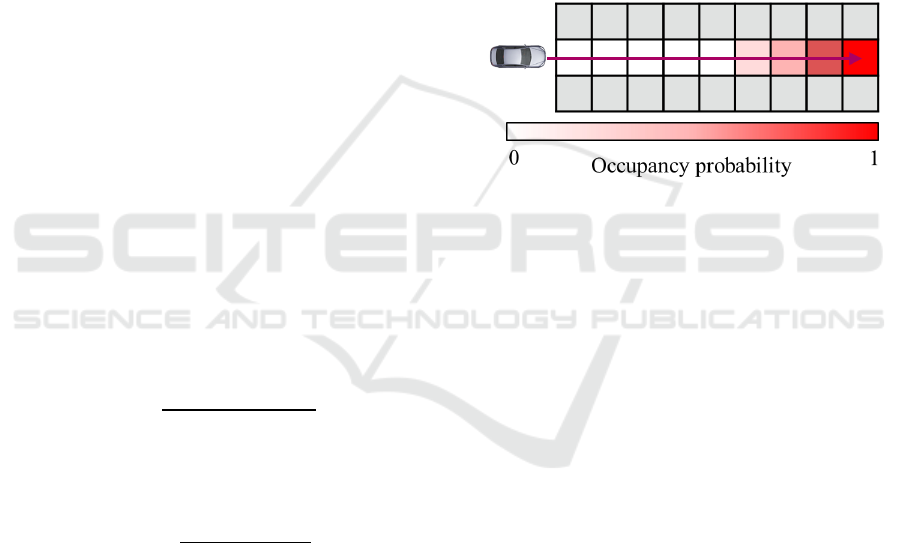
the LiDAR sensor detects an object, the grid, where
the target is located, is recognized as occupied (see
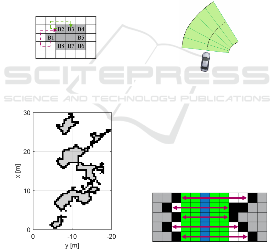
Figure 1). Between the occupied grid and LiDAR
sensor, the grids within a certain radial distance to
the LiDAR sensor are labelled as free. The
occupancy probability of the grids over the distance
threshold is computed with a linear function of the
distance between the grids and the target. The grids
(grey in Figure 1) without any measurement
information are marked as unknown.
Figure 1: LiDAR sensor model.
Since the radar sensors can sense objects behind
obstacles, a different sensor model is needed for the
computation of the occupancy probability.
Degerman, Pernstål and Alenljung (2016) extracted
Signal-to-noise ratio (SNR) and computed the
detection probability together with the Swerling 1
model. Using a static radar, Clarke et al. (2012)
calculated the occupancy probability as a function of
the reflection power, Fast Fourier Transform (FFT)
bin number of the range, as well as the bearing.
Werber et al. (2015) utilized the information about
the Radar Cross Section (RCS) to develop the
amplitude-based approach with occupancy grid
mapping. Considering the different properties and
modulations of the radar sensors, a general radar
sensor model can be created by converting the
reflection strength of the detection points into the
occupancy probability.
Since the previous automotive radar sensors
provide reflection data on the object level, the
occupancy grid map is often created from multiple
measurements in a limited area with the
Simultaneous Localization and Mapping (SLAM)
algorithm. Combining all the measurements, an
occupancy grid map of the whole measured area is
built, which helps to locate the vehicle position. The
grid map is also used to classify the stored objects
High Resolution Radar-based Occupancy Grid Mapping and Free Space Detection
71
on the cell level (Lombacher et al., 2017). However,
this approach is not applicable for the occupancy
grid mapping in the scope of real-time
measurements.
2.3 Free Space Detection
Based on the occupancy grid map, the free space
detection function is already developed in some
previous works with the LiDAR and camera sensor.
With the LiDAR sensor model the free space is
defined as a function of the distance between the
sensor and the target (Homm et al., 2010). The
further works focus on the road border recognition
with the classification ability in terms of the camera
sensor data (Badino, Franke and Mester, 2007)
(Andrew and Isard, 1998). Konrad, Szczot and
Dietmayer (2010) presented a road course estimation
approach using a multilayer laser scanner.
Lundquist, Schön and Orguner (2009) created a
curve fitting method to detect the road boundary on
the motorway. Schreier, Willert and Adamy (2016)
developed a parametric free space map, which
described a B-spline contour of arbitrarily shaped
outer free space boundaries around the ego vehicle
with additional attributes of the boundary type. In a
complex vehicle environment, a large number of the
curve parameters have to be estimated.
3 MEASUREMENT SETUP AND
DATA PREPARATION
A developed high performance radar system is
installed in the test vehicle and the measurement
data are recorded. The ego vehicle motion model is
simulated with the vehicle dynamic data from the
Controller Area Network (CAN) bus. The coordinate
systems of the vehicle and the grid map are adapted
with each other.
3.1 Radar Sensor
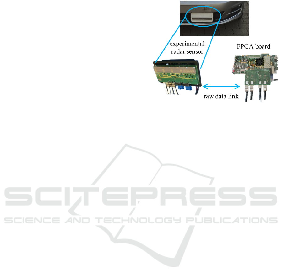
A 77 GHz FMCW experimental high performance
radar system is developed and mounted at the front
of the vehicle (see Figure 2) (Li, 2017). A Chirp
Sequence modulation with bandwidth B = 2.4 GHz,
observation cycle time T = 50 ms and a 16 channel
receive antenna array is applied.
Figure 2: Experimental radar sensor and FPGA board.
The measured raw data dimensions are 4096
samples, 1024 ramps and 16 channels. A Field-
Programmable Gate Array (FPGA) development
board is used to realize the signal processing
algorithms. A FFT over the samples is performed to
determine the distance information (range) of
detection points. For radial velocity detection, a
second FFT over the ramps is computed. In these
two dimensions a Chebyshev window is employed.
An Ordered Statistics Constant False Alarm Rate
(OS-CFAR) algorithm generates a threshold for the
target extraction of the calculated two dimensional
range-Doppler spectrum. The targets above the
threshold level are processed and their directions
(angle of arrival) are calculated with a Maximum
Likelihood algorithm.
A velocity threshold is set to select the relevant
target points from the static environment. The range
and angle of the reflection points in the radar polar
coordinate system are converted to
,
and
,
in
the Cartesian coordinate system. The middle of the
vehicle rear axle is defined as the origin point of the
coordinate system. The reflection amplitude
,
of
each point is computed with the signal processing
algorithm above. Thus, the information of reflection
points
at the time
t
can be represented by
=
,
,
,
,
,
,
,∈1…,
(3)
where is the number of the reflection points.
3.2 Vehicle Motion Model
Figure 3 shows the vehicle coordinate system
defined by ISO 8855:2011.
VEHITS 2018 - 4th International Conference on Vehicle Technology and Intelligent Transport Systems
72
Figure 3: Ego vehicle motion model.
From the CAN-Bus, the vehicle dynamic data
like velocity , acceleration and turn rate are
recorded. The ego vehicle motion is calculated based
on the Constant Turn Rate and Acceleration (CTRA)
model (Stellet et al., 2015) by
=
∙ ()
∙ ()
.
(4)
By integrating equation (4), the ego vehicle
position is calculated and presented by
=
,
,
,
.
(5)
Based on the ego vehicle position, the grid map
is tracked.
3.3 Grid Map Coordinate System
Generally the coordinate system of the occupancy
grid map can be defined by two methods:
1) Ground-fixed coordinate system. The ego
vehicle moves in this coordinate system at different
points. This method is suitable for the measurement
at limited place, like parking lot, otherwise a large
grid map is recommended to ensure the ego vehicle
is always in the map.
2) Vehicle-fixed coordinate system. The grid
map is shifted and rotated to keep the origin point
staying at the middle point of the vehicle rear axle.
However, undesirable offsets appear during the shift
and rotation. After the movement of the ego vehicle,
one single grid in the past map may occupy several
new grids in the shifted and rotated map, which
makes the grid map unstable or inaccurate.
To model and visualize the environment around
the vehicle in any places, the grid map coordinate
system needs to move with the ego vehicle like in
method 2. Meanwhile, some modifications are
applied to solve the offset problem. According to the
vehicle position, the grid map is just shifted with
integer rows and columns in x- and y- direction. The
rest difference between the origin point of the grid
map and the ego position
and
is retained (see
Figure 4). The orientation of the grid map is fixed by
using the ego vehicle direction from the first
measurement. During the vehicle motion the grid
map is not rotated, instead the orientation of the ego
vehicle
is saved. These values are used to update
the points in the coordinate system of the grid map.
With this method, the grid map is shifted in such a
way, that no offset is caused during tracking grid
map with the vehicle motion.
The length and width of the whole grid map is
adapted with the detection range of the radar sensor.
The size of a single grid is comparable with the
resolution of the radar sensor.
Figure 4: Grid map coordinate system.
The coordinates of the radar detection points in
the coordinate system of the ego vehicle are
converted into the grid map coordinate system by
,
,
=
−
,
,
+
.
(6)
4 OCCUPANCY GRID MAPPING
Depending on the position, the radar reflection
points are assigned into the corresponding grids. In
each time step, the occupancy grid is updated
considering the current measured value by the radar
sensor and the previous value of the grid. This leads
to reduced measurement uncertainties and errors,
since the real obstacles are typically detected in
continuous measure cycles and mapped in the same
grids over time.
The reflection strength of every new point is
converted into a normalized value. Combining the
values of all points in one single cell, the detection
High Resolution Radar-based Occupancy Grid Mapping and Free Space Detection
73
probability in the cell is calculated. In each cycle
this probability is computed and combined with each
other to gain the a posteriori probability, which
builds the final valid occupancy grid map. In the
following part, the approach of the detection
probability and a posteriori probability is introduced.
4.1 Detection Probability
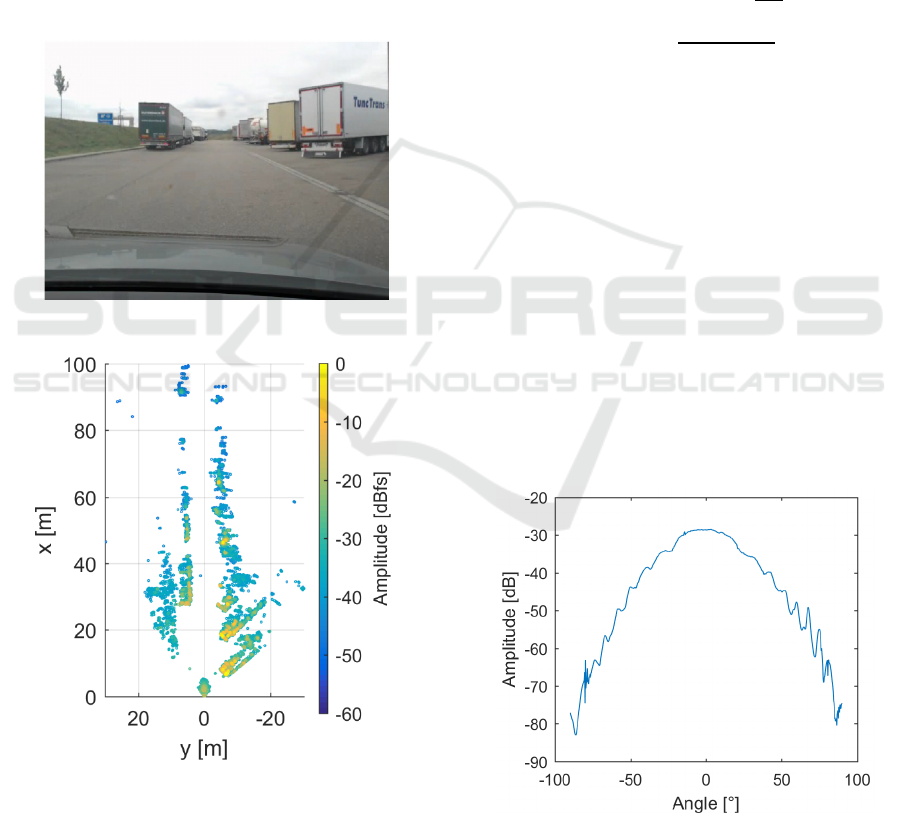
In Figure 5, an image of one measurement cycle at a
parking spot is shown, its corresponding bird's-eye
view of the raw radar data is presented in Figure 6.
In the next part, the reflection amplitudes of all
detection points are converted to the detection
probability in each grid.
Figure 5: Image of real scenario at a parking spot.
Figure 6: Bird's-eye view of radar reflection points.
4.1.1 Free-Space Loss Compensation
The free-space loss describes the decrease of the
power density during the propagation of
electromagnetic waves in free space according to the
distance law, without taking additional attenuating
factors (e.g. rain or fog) into account. The reflection
amplitude is weakened with the increasing distance
to the radar sensor.
In order to make the reflection strength and the
converted detection probability of the obstacles
independent of the distance, the free-space loss is
compensated. The relationship between the
reflection amplitude and the radial distance of the
points is given in the equation (7). The amplitudes of
all points are converted to the equivalent value
,
at a reference distance
to the radar sensor.
,
=
,
−40
,
(7)
with
,
=
,
+
,
4.1.2 Antenna Gain Compensation
The reflection amplitudes of the points are
additionally influenced by the angle between the
target and the radar sensor, which is related to the
antenna gain. The different antenna gain pattern is
compensated, to achieve a reflection amplitude that
is independent of the angle of arrival. In order to
know the relationship between the amplitude and the
angle of the reflection point, a corner reflector is
placed at the same distance but with different angles
to the radar sensor and the reflection amplitudes of
the reflector at different angles are measured (see
Figure 7). With this antenna pattern the amplitudes
of all points are converted to an isotropic value that
eliminates any angular dependency.
Figure 7: Antenna gain empirical characteristic curve.
4.1.3 Reflection Amplitude Normalization
The reflection amplitude is a relative value and
VEHITS 2018 - 4th International Conference on Vehicle Technology and Intelligent Transport Systems
74
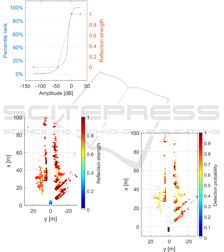
varies with different signal processing algorithms
and parameters. However, the relationship of the
amplitude between different points always presents
the relative reflection strength. Therefore, the
compensated amplitude is normalized to a value
between 0 and 1. For each measurement cycle all the
points are sorted by their amplitudes (see Figure 8).
Figure 8: Distribution and normalization of reflection
amplitude.
Figure 9: Normalised reflection amplitude.
If the maximum amplitude value is set to 1 for
the reflection strength and the minimum amplitude
value to 0, an unsuitable scale is applied, since some
points have an extreme value. Due to this, the 10%
maximum value is normalized to 1 and the 10%
minimum value to 0. The reflection amplitude
between them is converted according to a linear
function to the value. Thus, the reflection strength of
all points is normalized (see Figure 9).
4.1.4 Detection Probability in Single Grid
After the compensation and normalization of the
reflection amplitude the points are allocated into the
grids. Each grid can be occupied by several points
with different reflection strength. The detection
probability in one single grid can be calculated with
the reflection strength of all points or the point
number in this grid. In the grid some points with
high reflection strength are detected from one object,
while some points with a low reflection strength are
reflected from another object nearby because of the
antenna side lobes. The influence of those points
with low reflection strength should be ignored,
otherwise a low detection probability is computed by
calculating the average reflection strength in one
grid. Besides, the point number in every grid
depends strongly on the size of the grid.
For the reasons above, only the points with 20%
maximum reflection strength values in each grid are
considered in the calculation. Their average
reflection strength value is defined as the detection
probability in the grid. In Figure 10 the detection
probability of all grids in one measurement cycle is
depicted.
Figure 10: Detection probability (Ego vehicle is near
origin point).
High Resolution Radar-based Occupancy Grid Mapping and Free Space Detection
75
4.2 A Posteriori Probability
The radar sensor model converts the reflection
strength to the detection probability, which is
different from the LiDAR sensor model, so the
equation (2) is modified.
At first, the detection probability is scaled to a
value between 0.5 and 1 with the equation (8),
otherwise the reflection strength under 0.5, which is
also from the obstacles, leads to the reduction of the
log odds ratio of the a posteriori probability.
(
|
,
)
=0.5 + 0.5 ∗
(
|
,
)
(8)
However, with the scaling of the detection
probability, the a posteriori probability is increased
every time when the data from the new measurement
cycle are calculated. This problem is solved by the
degradation factor
k
. Then the log odds ratio of the a
posteriori probability is computed with the equation
ℓ
=∗ℓ
+
(|
,
)
1−
(|
,
)
.
(9)
With the movement of the ego vehicle, the grids
with the value of occupancy probability are shifted.
Thus, the grid holds the detection probability based
on the radar data in the current cycle and the
occupancy probability in the previous cycles. The
previous radar data should have less influence on the
final occupancy probability than the new data. With
the degradation factor
k
, the log odds ratio of the
occupancy probability ℓ
is reduced with respect
to time. Therefore in each cycle the value of
occupancy probability in the grids is reduced with
the degradation factor at first and then increased
with the current detection probability.
The log odds ratio ℓ
in the grid is normalized to
the value between 0 and 1, which indicates the a
posteriori occupancy probability. The maximum and
minimum limits are decided with a prognosis
method: an object is located in one grid and detected
with the same detection probability
in every
cycle. After
n
measurement cycles, the grid is
assumed to be 100% occupied. The current log odds
ratio value is set to be upper limit ℓ
,
, which is
represented by value 1 of the a posteriori probability.
ℓ
,
can be calculated by
ℓ
,
=
∗log
1−
.
(10)
In the following
m
cycles, no point with any
reflection is detected in this grid. The grid is
assumed to be free again. The current log odds ratio
value is defined as the lower limit ℓ
,
, which is
represented by value 0 for the a posteriori
probability. ℓ
,
can be calculated by
ℓ
,
=ℓ
,
∗
.
(11)
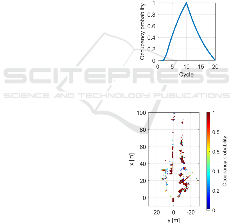
The log odds ratio between the upper and lower
limits is converted to the value between 0 and 1. In
Figure 11 the change curve of the occupancy
probability with the measurement cycle in the
prognosis (
=0.9,==10) is shown. In the
10
th
cycle the occupancy probability reaches the
maximum value, then decreases and appears in the
20
th
cycle at the minimum.
Figure 11: Change curve of occupancy probability in
prognosis.
4.3 Results
Figure 12: Occupancy grid map at a parking spot.
VEHITS 2018 - 4th International Conference on Vehicle Technology and Intelligent Transport Systems
76
The a posteriori probability stands for the final
occupancy probability in each cycle. In Figure 12
the occupancy grid map from
the measurement at a
parking spot is shown, where several trucks and vans
are parked (see Figure 5). In the occupancy grid map
the contours of the trucks are recognized, although
they are parked close to each other. The occupancy
probability in the area of trucks is almost 1 and the
grids between them have an occupancy probability
of 0. This occupancy grid map represents correctly
the static environment.
4.4 Amplitude Grid Mapping
The amplitude grid mapping is another common
method to map the grid, which normalizes the
maximum value of reflection amplitude over time in
every grid into the occupancy probability. In Figure
13, an example of the amplitude grid mapping is
shown. In contrast to the occupancy grid mapping,
the measurement noise is not filtered and presented
in the grid map, since only the maximum value is
considered and the duration cycle of the
measurement value is ignored. Because of the
measurement noise, in some existing free space a
high occupancy probability is computed, which
disturbs the free space detection.
Figure 13: Example for amplitude grid mapping.
5 FREE SPACE DETECTION
The free space detection in the whole area around
the vehicle is not achievable, because no data are
captured out of the detection range and aperture of
the radar sensor or behind some large obstacles. For
the vehicle motion planning the field of interest
(FOI) is the area along the possible trajectory. At
first the occupancy status in all grids is determined
in order to create a binary grid map. With the
clustering method, the occupied areas, which are
caused by the constant and strong reflection points
from the measurement errors, are defined as free
space again. Based on the border recognition
algorithm, the boundary of the occupied areas is
detected, which realizes the free space detection
along the vehicle trajectory.
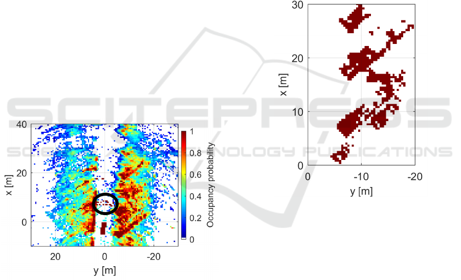
5.1 Occupancy Status Determination
Before detecting the free space, it should be
determined, whether the grids are occupied or not.
The easiest way is to use a constant threshold of the
occupancy probability, the occupancy status of the
grids is decided, so that the occupancy grid map can
be converted to a binary grid map (see Figure 14).
Figure 14: Binary grid map with threshold of occupancy
probability (red: occupied grid, white: free grid).
However, the occupancy status of some grids has
a mismatch with the respective value due to the
features of the radar sensor and the OS-CFAR
algorithm. From one object a lot of reflection points
are detected and assigned in the different grids.
Some points among them have low refection
amplitudes, so that the occupancy probability of the
corresponding grids is close to zero. Those grids are
detected as free space, which actually belong to the
obstacles. Here two methods are developed, in order
to recognize the grids belonging to the obstacles but
with low occupancy probability as occupied.
1) The grids with an occupancy probability
lower than the threshold are considered. The amount
of the grids in the neighbourhood, which have much
higher occupancy probability than the selected grid,
is calculated (see grids N in Figure 15, image on the
High Resolution Radar-based Occupancy Grid Mapping and Free Space Detection
77
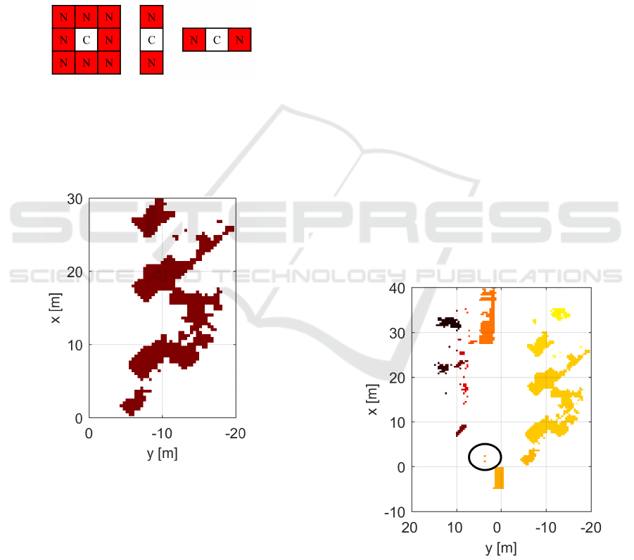
left). If this amount is larger than a threshold, the
selected grid (gird C in Figure 15) is set to be
occupied. Using this method, the grids with a lower
occupancy probability in the inside and border area
of obstacles are recognized as occupied.
2) The grids with zero occupancy probability are
handled. If the two “sandwiched” grids (see grids N
in Figure 15, middle and right) have a high
occupancy probability and are declared as occupied,
the selected grid is set to be occupied. Thus,
especially the grids with zero occupancy probability
in the inside area of obstacles are detected as
occupied.
Figure 15: Neighbour grids (C: centre grid. N: neighbour
grid).
Using the methods above, the occupancy status
of all grids can be determined. An example of the
results is shown in Figure 16.
Figure 16: Processed binary grid map.
5.2 Clustering Binary Grids
With the occupancy grid mapping, the random
measurement noise is filtered. However, some
reflection points are caused by the strong objects
nearby or the measurement errors. In the binary grid
map the points usually occupy some areas with
small size outside the obstacles, which are named as
outliers. Using the threshold of the connected
occupied area size, the outliers are filtered.
In order to calculate the size of the connected
occupied areas, it is necessary to group the binary
grids at first. Three popular clustering algorithms are
discussed here:
1) K-Means (Lloyd, 1982). The partitions of the
grids are divided into a predefined number of
clusters in which each grid belongs to the cluster
with the nearest mean. Since the environment
around the vehicle changes all the time, it is not
efficient to predefine the number of clusters.
2) Density-Based Spatial Clustering of
Applications with Noise (DBSCAN) (Ester et al.,
1996). The grids are grouped together and classified
into core, border and noise grids depending on the
number of occupied neighbour grids. The noise grids
here are recognized as outliers. In order to filter the
noise grids precisely, a relative low distance
threshold between the grids and a relative high
threshold of the grid number is selected. However,
the calculation time is very long, because it is a
quadratic function of the grid number in the worst
case.
3) Connected component labelling (CCL)
(Rosenfeld and Pfaltz, 1999) (He, Chao and Suzuki,
2008). The connected occupied grids in binary grid
map is detected and clustered. It is not necessary to
predefine any parameters. Additionally it takes
significantly less computational burden than
DBSCAN. For this reason, CCL is chosen as the
clustering algorithm here.
Figure 17: Clustering with CCL algorithm.
The number of the grids in each cluster is
calculated. With a number threshold the outliers are
found and the grids from the outlines are marked as
free again. This processing step is meaningful,
VEHITS 2018 - 4th International Conference on Vehicle Technology and Intelligent Transport Systems
78
because some outliners are located directly in front
of the vehicle, where belongs to the FOI. In Figure
17 an example of the clustering result with CCL
algorithm is demonstrated. The grids in the black
circle are clustered and then defined as free again.
5.3 Border Recognition
The boundaries of the clustered and occupied binary
grids are mostly relevant for the free space detection.
The Moore-Neighbour Tracing (MNT) algorithm is
introduced here to recognize the border of the
occupied areas (Gonzalez et al., 2004). In Figure 18
the MNT algorithm is described. Starting from a
random occupied grid B1, the next occupied
neighbour grid in the clockwise direction B2 is
searched. The iteration loop terminates when the
initial grid is visited for a second time.
Figure 18: MNT Algorithm (B: border grid).
All reached grids are labelled as border grids,
which helps to detect the free space along the
trajectory. In Figure 19 an example of the border
recognition result is shown.
Figure 19: Border recognition (black: border grid, grey:
occupied grid).
5.4 Interval-based Free Space Model
The free space along the vehicle trajectory is defined
by the narrowest distance between the vehicle future
possible position and the border of the occupied
areas.
At first the trajectory of the ego vehicle is calculated
with the current dynamic data based on the CTRA
model, where the vehicle positions and orientations
along the trajectory are computed. It is also possible
to calculate the vehicle trajectory with any
manoeuvres. The vehicle trajectory is defined as
baseline and extended with a certain distance
considering the orientation at each position to an
area, which is similar to a sector and defines the FOI
along the trajectory (see Figure 20).
Figure 20: FOI and intervals along the trajectory.
Thereafter the FOI is divided into intervals with
a certain length along the trajectory. The interval is
always perpendicular to the vehicle orientation at
each point. The length of one single interval is defi-
ned as a function of the vehicle velocity, because a
wider free space is needed with increasing velocity.
In order to realize the interval-based free space
model, the grids, in which the vehicle positions in
the FOI are located, are selected to be the baseline
grids. The grids on the left and right side of the
baseline grids are visited with the Bresenham's line
algorithm, which is located in the perpendicular
direction to the vehicle orientation at each position
(see Figure 21).
Figure 21: Free space detection in one interval (Blue:
baseline grid, green: free space grid, black: border grid,
grey: occupied grid).
High Resolution Radar-based Occupancy Grid Mapping and Free Space Detection
79
The occupied grid with the smallest distance to
each baseline grid is searched. Then this distance is
defined as the width of the free space interval. The
grids in the interval, which are closer to the baseline
grids, are labelled as free space. Similarly, the width
of all the intervals can be calculated, so that the free
space along the vehicle trajectory is detected.
5.5 Results
In Figure 22 an example of the free space detection
at the parking spot is shown. On the left side in front
of the vehicle, more free space exists than on the
right side, which means, the evasive trajectory to left
is more feasible than right. Additionally the parking
slots between the trucks are recognized as free
space, which helps to generate the parking
manoeuvre.
Figure 22: Example for free space detection.
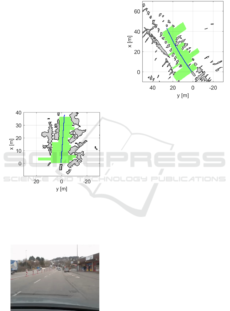
In Figure 23 and Figure 24 another example on
the public road is shown. There are several warning
posts at the left side of the road, which are separately
detected as obstacles in the map. The distance
between the warning posts is recognized as free
space.
Figure 23: Image for measurement on public road.
Figure 24: Free space detection on public road.
6 CONCLUSIONS
This paper presents an approach of the occupancy
grid mapping and free space detection based on the
high resolution radar sensors.
The positions and reflection amplitudes of the
target points are detected with radar sensor and used
as input data for the occupancy grid mapping. The
reflection amplitudes are compensated according to
the free-space loss and antenna pattern gain, and
finally normalized. Based on the positions, the
detected points are assigned to the corresponding
grids. The detection probability of the individual
cells is calculated as the function of the reflection
strength of the detection points. With the movement
of the ego vehicle, the value of the grids is degraded
and then combined with the new data to compute the
a posteriori occupancy probability. Thus, an
occupancy grid map is updated over the course of
time.
Thereafter the occupancy grid map is converted
to the binary grid map. The grids in the obstacle
areas are searched and labelled as occupied
depending on the neighbour grids. Using the CCL
algorithm, the connected occupied grids are
clustered, in order to eliminate the outliers. With the
MNT algorithm the border of the clustered occupied
grids is recognized. Finally an interval-based free
space is detected utilizing the Bresenham's line
algorithm. According to the measurement results the
detected free space and obstacles with the approach
above match with the real scene.
VEHITS 2018 - 4th International Conference on Vehicle Technology and Intelligent Transport Systems
80

ACKNOWLEDGEMENTS
This work has received funding from the European
Community’s Eighth Framework Program
(Horizon2020) under grant agreement no. 634149
for the PROSPECT project and funding from the
German Federal Ministry for Economic Affairs and
Energy for the iFUSE project. The PROSPECT and
iFUSE consortium members express their gratitude
for selecting and supporting these two projects.
REFERENCES
Andrew, B. and Isard, M., (1998). Active Contours: The
Application of Techniques from Graphics, Vision
Control Theory and Statistics to Visual Tracking of
Shapes in Motion. 1st ed. London: Springer.
Badino, H., Franke, U. and Mester, R., (2007). Free Space
Computation Using Stochastic Occupancy Grids and
Dynamic Programming. In International Conference
on Computer Vision (ICCV), Workshop on Dynamical
Vision, Rio de Janeiro.
Badino, H., Mester, R., Vaudrey, T., Franke, U. and
Daimler AG, (2008). Stereo-based Free Space
Computation in Complex Traffic Scenarios. In IEEE
Southwest Symposium on Image Analysis and
Interpretation (SSIAI), Santa Fe, pp. 189-192.
Clarke, B., Worrall, S., Brooker, G. and Nebot, E., (2012).
Sensor Modelling for Radar-Based Occupancy
Mapping. In IEEE/RSJ International Conference on
Intelligent Robots and Systems (IROS), Vilamoura, pp.
3047-3054.
Degerman, J., Pernstål, T. and Alenljung, K., (2016). 3D
Occupancy Grid Mapping Using Statistical Radar
Models. In IEEE Intelligent Vehicles Symposium (IV),
Gothenburg, pp. 902-908.
Elfes, A., (1989). Using Occupancy Grids for Mobile
Robot Perception and Navigation. In Computer, vol.
22, no. 6, pp. 46-57.
Ester, M., Kriegel, H. P., Sander, J. and Xu, X., (1996). A
Density-Based Algorithm for Discovering Clusters in
Large Spatial Databases with Noise. In Proceedings of
the Second International Conference on Knowledge
Discovery and Data Mining, Portland, pp. 226-331.
Gonzalez, R. C., Woods, R. E. and Eddins, S. L., (2004).
Digital Image Processing Using MATLAB, Lexington:
Pearson Prentice Hall.
He, L., Chao, Y. and Suzuki, K., (2008). A Run-Based
Two-Scan Labeling Algorithm. IEEE Transactions on
Image Processing, 17(5), pp. 749-756.
Homm, F., Kaempchen, N., Ota, J. and Burschka, D.,
(2010). Efficient Occupancy Grid Computation on the
GPU with LiDAR and Radar for Road Boundary
Detection. In IEEE Intelligent Vehicles Symposium
(IV), San Diego, pp. 1006-1013.
Konrad, M., Szczot, M. and Dietmayer, K., (2010). Road
Course Estimation in Occupancy Grids. In IEEE
Intelligent Vehicles Symposium (IV), San Diego, pp.
412-417.
Li, M., (2017). High-Resolution Radar Based
Environment Perception and Maneuver Planning. In
CTI Symposium on Automated Driving, Future
Mobility and Digitalization (ADFD), Hannover.
Lloyd, S., (1982). Least Squares Quantization in PCM.
IEEE Transactions on Information Theory, 28(2), pp.
129-137.
Lombacher, J., Laudt, K., Hahn, M., Dickmann, J. and
Wöhler, C., (2017). Semantic Radar Grids. In IEEE
Intelligent Vehicles Symposium (IV), Los Angeles, pp.
1170-1175.
Lundquist, C., Schön, T. B. and Orguner, U., (2009).
Estimation of the Free Space in Front of a Moving
Vehicle. In SAE World Congress & Exhibition,
Detroit.
Meinl, F., Stolz, M., Kunert, M. and Blume, H., (2017).
An Experimental High Performance Radar System for
Highly Automated Driving. In IEEE MTT-S
International Conference on Microwaves for
Intelligent Mobility (ICMIM), Nagoya, pp. 71-74.
Moravec, H. and Elfes, A., (1985). High Resolution Maps
from Wide Angle Sonar. In Proceedings of IEEE
International Conference on Robotics and
Automation, St. Louis, pp. 116-121.
Mouhagir, H., Cherfaoui, V., Talj, R., Aioun, F. and
Guillemard, F., (2017). Using Evidential Occupancy
Grid for Vehicle Trajectory Planning Under
Uncertainty with Tentacles. In IEEE 20th
International Conference on Intelligent
Transportation Systems (ITSC), Yokohama.
Nuss, D. (2017). A Random Finite Set Approach for
Dynamic Occupancy Grid Maps. PhD. University of
Ulm.
Rosenfeld, A. and Pfaltz, J. L., (1999). Sequential
Operations in Digital Picture Processing. Journal of
the ACM, 13(4), pp. 471-494.
Schreier, M., Willert, V. and Adamy, J., (2016). Compact
Representation of Dynamic Driving Environments for
ADAS by Parametric Free Space and Dynamic Object
Maps. IEEE Transactions on Intelligent
Transportation Systems, 17(2), pp. 367-384.
Stellet, J. E., Straub, F., Schumacher, J., Branz, W. and
Zöllner, J. M., (2015). Estimating the Process Noise
Variance for Vehicle Motion Models. In IEEE 18th
International Conference on Intelligent
Transportation Systems (ITSC), Las Palmas, pp. 1512-
1519.
Weiss, T., Schiele, B. and Dietmayer, K., (2007). Robust
Driving Path Detection in Urban and Highway
Scenarios Using a Laser Scanner and Online
Occupancy Grids. In IEEE Intelligent Vehicles
Symposium (IV), Istanbul, pp. 184-189.
Werber, K., Rapp, M., Klappstein, J., Hahn, M.,
Dickmann, J., Dietmayer, K. and Waldschmidt, C.,
(2015). Automotive Radar Gridmap Representations.
In IEEE MTT-S International Conference on
Microwaves for Intelligent Mobility (ICMIM),
Heidelberg, pp. 1-4.
High Resolution Radar-based Occupancy Grid Mapping and Free Space Detection
81
