Base Algorithms of Environment Maps and Efficient Occupancy Grid
Mapping on Embedded GPUs
J
¨
org Fickenscher
1
, Frank Hannig
1
, J
¨
urgen Teich
1
and Mohamed Essayed Bouzouraa
2
1
Department of Computer Science, Friedrich-Alexander University Erlangen-N
¨
urnberg (FAU), Germany
2
Concept Development Automated Driving, AUDI AG, Ingolstadt, Germany
Keywords:
Autonomous Driving, Environment Maps, GPGPU.
Abstract:
An accurate model of the environment is essential for future Advanced Driver Assistance Systems ( ADAS s).
To generate such a model, an enormous amount of data has to be fused and processed. Todays Electronic
Control Units ( ECU s) struggle to provide enough computing power for those future tasks. To overcome these
shortcomings, new architectures, like embedded Graphics Processing Units ( GPU s), have to be introduced. For
future ADAS s, also sensors with a higher accuracy have to be used. In this paper, we analyze common base
algorithms of environment maps based on the example of the occupancy grid map. We show from which sensor
resolution it is rational to use an (embedded) GPU and which speedup can be achieved compared to a Central
Processing Unit ( CPU ) implementation. A second contribution is a novel method to parallelize an occupancy grid
map on a GPU, which is computed from the sensor values of a lidar scanner with several layers. We evaluate our
introduced algorithm with real driving data collected on the autobahn.
1 INTRODUCTION AND
RELATED WORK
Motivation: Since the last years, there is an enormous
hype about autonomous driving and ADAS s. To make
it happen, e.g., driving autonomously on a highway,
a vehicle needs an accurate model of its environment.
These models have to contain all static and dynamic
objects in the vehicle surroundings, as well as the own
vehicle position. To create such a model, sensors with
a high resolution are necessary. These sensors deliver
enormous amounts of data, which have to be fused
and processed to create an accurate environment map.
Nowadays, the processors in ECU s, which are mostly
single-core CPU s, struggle to provide enough com-
puting power for these tasks. Here, new emerging
architectures appear. One of the most promising is the
use of GPU s in automotive ECU s. Today’s hardware
performance gains are mostly achieved through more
cores and not through a higher single-core performance.
Here, GPU s perfectly fit in, with their hundreds of cores
in embedded systems compared with mostly quad-core
CPU s in embedded systems. To use such architectu-
res, it is necessary to switch from the predominant
single-threaded programming model to a multi-threaded
programming model. Thus, the software has to be
adjusted, parallelized were possible or entirely new
written for these platforms. Another key point is that
not only new hardware platforms but also new sensors
with a higher accuracy are necessary for future ADAS s.
One important research question is, we look into in this
paper, how the algorithms scale for larger sensors, and
what is the sweet spot of the architecture (CPU/GPU)
and mapping. Often, if an environment map is created,
there are several base algorithms, which are necessary,
no matter which type of environment map is created.
As a first contribution, we analyze in this paper, how
the base algorithms scale with different sensor resolu-
tions on different hardware platforms, which is very
important knowledge for Original Equipment Manufac-
turers ( OEM s). In former times, sensors scanned only
one vertical layer of the environment. However, they
have not only an increased resolution in the horizontal
but recently also in the vertical direction. Since the me-
asurements in the vertical direction may be dependent,
it is not easy to evaluate such sensor measurements in
parallel on a GPU . We purpose a novel parallel evalua-
tion of lidar scanner data on the example of the very
well-known environment map, the occupancy grid map.
To show the capability of our approach, we evaluate
it with collected real-time data by an experimental car.
In the next paragraph, we discuss related work. In
Section 2, we give an overview of the base algorithms
of environment maps and introduce our new method for
the parallelization of an occupancy grid map on a GPU .
Subsequently, we evaluate our approach in Section 3.
Finally, we conclude our paper in Section 4.
Related Work: Creating environment maps, like the
298
Fickenscher, J., Hannig, F., Teich, J. and Bouzouraa, M.
Base Algorithms of Environment Maps and Efficient Occupancy Grid Mapping on Embedded GPUs.
DOI: 10.5220/0006677302980306
In Proceedings of the 4th International Conference on Vehicle Technology and Intelligent Transport Systems (VEHITS 2018), pages 298-306
ISBN: 978-989-758-293-6
Copyright
c
 2019 by SCITEPRESS – Science and Technology Publications, Lda. All rights reserved

occupancy grid map, introduced by Elfes (Elfes, 1989)
and Moravec (Moravec, 1988), is a common problem
in robotics. They used their approach to describe the
environment, which was static, for a mobile robot.
Also, grid maps are used in robotics for Simultaneous
Localization and Mapping ( SLAM ) problems like in
(Grisettiyz et al., 2005) or multiple object tracking
(Chen et al., 2006). Most of the approaches use only a
2D occupancy grid, but some works extended it to a
third dimension (Moravec, 1996). The problem with
3D methods is the high memory consumption, which
was addressed by (Dryanovski et al., 2010). Since the
basic idea of robotics and autonomous vehicles is very
similar, it is not surprising that the concept of occupancy
grid maps was also introduced to the automotive sector.
The difference to the automotive context is, that for
robotics often a static map is created only once, whereas
for vehicles the map has to be continuously updated
due to the dynamic environment. In (Badino et al.,
2007), the authors introduced an occupancy grid for
the automotive domain to compute the free space of
the environment. Occupancy grid maps are also used
for lane detection (Kammel and Pitzer, 2008) or path
planning (Sebastian Thrun, 2005). Often laser range
finders are used to create occupancy grid maps (Homm
et al., 2010) (Fickenscher et al., 2016), as we consider
in this paper, but it is also possible to use radar sensors
(Werber et al., 2015) to create such maps. Since creating
occupancy grid maps can be very compute-intensive, it
was parallelized on a GPU (Homm et al., 2010). They
used in their approach a desktop PC, as proof of con-
cept. However, space and energy requirements are far
away from a realistic ECU . In this paper, we use an
embedded platform, which is much more similar to a
later ECU design. Yguel et al. (Yguel et al., 2006) used
several laser range finders, but only with one vertical
layer and they did their experiments also on a desktop
computer. In (Fickenscher et al., 2016), the occupancy
grid map was parallelized on an embedded GPU . In
this approach, a laser sensor with only one layer in the
vertical was used. In this paper instead, a sensor with
several vertical layers is used. Hereby the accuracy of
the occupancy grid map is enormously increased but
also the computational effort rises proportionally.
2 FUNDAMENTALS
In this section, a brief overview of creating environment
maps, especially an occupancy grid map is given. Then,
our very efficient algorithm to create an occupancy grid
is described and its parallelization. Also, the specific
properties of embedded GPU s are shortly summarized.
Further, differences in parallelizing the algorithm on a
Host (CPU)
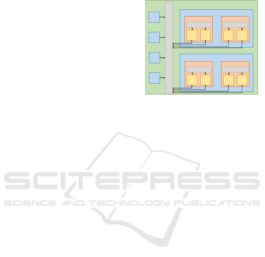
Grid 0
Block (0,0)
Shared Memory
Thread
(0,0)
Thread
(1,0)
Block (1,0)
Shared Memory
Thread
(0,0)
Thread
(1,0)
M
e
m
o
r
y
Grid 1
Block (0,0)
Shared Memory
Thread
(0,0)
Thread
(1,0)
Block (1,0)
Shared Memory
Thread
(0,0)
Thread
(1,0)
Device (GPU)
CPU 0
CPU 2
CPU 3
CPU 1
Figure 1: Structural overview of the CUDA programming
model for an embedded GPU.
GPU, instead on a CPU are described.
2.1 Programming an Embedded GPU
The main purpose of GPU s has been rendering of com-
puter graphics, but with their steadily increasing pro-
gramming and memory facilities, GPU s recently be-
come attractive for also accelerating compute-intensive
algorithms from other domains. GPU s show their
strengths, if the algorithm has a high arithmetic density
and could be parallelized in a data-parallel way. Ho-
wever, the hardware architecture of a GPU and a CPU
is quite different. A GPU embodies at hardware level
several streaming processors, which further contain
processing units. Such a streaming processor manages,
spawns, and executes the threads. Those threads are
managed in groups of 32 threads, so-called warps. In a
warp, every thread has to execute the same instruction
at the same time. E.g., if there is a branch, for which
only half of the threads, the statement is evaluated true,
the other half of the threads has to wait. As illustrated
in Figure 1, threads are combined to logical blocks,
and these blocks are combined to a logical grid. In
2006 (NVIDIA Corp., 2016b), Nvidia introduced the
framework CUDA to ease the use of GPU s for general
purpose programming. Program blocks, which should
be executed in parallel, are called kernels. Those kernels
can be executed over a range (1D/2D/3D) specified by
the programmer. For a range, which has n elements,
n threads are spawned by the CUDA runtime system.
The programming model for the parallelization of an
algorithm is also different. On a CPU , parallel threads
are executed on different data, and every thread pro-
cesses different instructions. On a GPU instead, every
thread executes the same instruction at the same time on
different data. This model is called Single Instruction
Multiple Threads ( SIMT ). The main difference bet-
Base Algorithms of Environment Maps and Efficient Occupancy Grid Mapping on Embedded GPUs
299

coordinate transformation:
-intrinsic calibration (sensor model)
-extrinsic calibration (sensor model)
ego-motion compensation
prediction of ego-motion
map update with association of
measurements
laser measurement
(fusion model)
prediction of laser measurement
Figure 2: Overview of the sub-algorithms which are necessary to create an environment map.
ween a discrete desktop GPU and an embedded GPU
is the memory system. On an embedded GPU , like
illustrated in Fig. 1, there is no separation between the
main memory of the system and the GPU memory, like
on a desktop computer. So on an embedded, GPU no
data has to be explicitly copied from the main memory
to the GPU memory to execute an algorithm on that
data on the GPU.
2.2 Base Algorithms of ADAS
Environment maps represent the surrounding of a car
and are always necessary for automated driving systems.
No matter which environment map is used, there are
a few base algorithms, which are always necessary,
e.g., the compensation of the ego-motion, coordinate
transformations and updating the environment map. In
Figure 2 an overview of the different base algorithms,
which are necessary to create an environment map,
are given. The brown arrows indicate the predict and
update step of the Kalman filter (Kalman, 1960), which
is independent of the other base algorithms. In the
following, these algorithms are further described.
2.2.1 Coordinate Transformation
To create an environment map out of the sensor measure-
ments, the characteristics of the sensor model have to be
considered. A sensor model consists of intrinsic and the
extrinsic parameters. For example, if a fisheye camera is
used, the intrinsic calibration process is to transform the
stream with a strong visual distortion into a stream with
straight lines of perspective. Since the sensors have dif-
ferent positions on the vehicle, all the measurements of
the sensors have to be transformed into one coordinate
system. This is the extrinsic calibration process. First,
they have to be transformed into Cartesian coordinates
because that is the coordinate system of the environment
map. The sensor measurements of, e.g., laser scanners
are normally in polar coordinates r and ϕ . Therefore, the
measurements have to be transformed from polar to Car-
tesian coordinates with x = r cosϕ and y = r sinϕ . The
fisheye camera has a spherical coordinate system and
with x = r sinΘcos ϕ , y = r sinΘsin ϕ and z = r cosΘ
it can be transformed to Cartesian coordinates. The
origin of the coordinate system for environment maps is
often set to the middle of the rear axle of the vehicle.
So all the coordinate systems with different origins
have to be transformed to a coordinate system with one
origin. We use homogeneous coordinates to do this
transformation.
2.2.2 Ego-motion Compensation
By creating an environment map, it is also necessary
to compensate the ego-motion of the own vehicle. In
principle, there are two approaches to do that. One is to
compensate the sensor measurements by the ego-motion
directly. For that, usually homogeneous coordinates
are used, because the translation and rotation can be
done with one matrix. The matrix is used for every laser
beam to compensate the ego-motion.
The other method is to shift the environment map by
the ego-motion of the own vehicle. E.g., if an occupancy
grid map is used the ego-motion can be compensated by
rotating the vehicle on the map and shifting two pointers,
one for the movement in x-direction and one for the
movement in y-direction, like explicitly described in
(Fickenscher et al., 2016).
2.2.3 Fusion Model
To get a detailed knowledge about the vehicle envi-
ronment, different sensors are necessary. The measu-
VEHITS 2018 - 4th International Conference on Vehicle Technology and Intelligent Transport Systems
300

rements of different sensors have to be put together,
to have an entire picture of the environment in one
map. In the fusion model, this step is done. First, the
different data has to be synchronized in time, because
different sensors have a different update interval. In a
second step, the data has to be merged together. That is
the speed of a vehicle, measured by a radar sensor, is
combined with the detected vehicle by a laser scanner.
2.2.4 Kalman Filter
Sensor measurements often contain some noise or other
inaccuracies, e.g., statistical outliers. The Kalman
filter (Kalman, 1960) is used to estimate values, e.g.,
the speed of the own vehicle, based on several past
measurements. Those estimations are combined with
the actual measurement. As a result of this the actual
measurement is smoothed, to get rid of challenges
mentioned above.
2.2.5 Update Environment Map
To update an environment map, the new sensor measure-
ments have to be entered into the old map. Therefor, it
is necessary to associate the objects in the environment
map with the new measurements from the sensor. It has
to be decided, which measurement belongs to which ob-
ject or if there is a belonging object to a measurement or
not and a new one has to be created. A simple algorithm
for this challenge would be for example Global Nearest
Neighbor ( GNN ), based on the work of Cover and Hart
(Cover and Hart, 2006). Here, for every already tracked
object the distance to all measured objects is calculated
and then, the measurement is associated with the closest
distance to a tracked object. A more sophisticated ap-
proach is the probabilistic data association filter ( PDAF )
(Bar-Shalom et al., 2009) (Musicki and Evans, 2004).
Commonly, a probabilistic data association ( PDA ) algo-
rithm computes the association probabilities, taking into
account the uncertainties of the measurement, to the
targets being tracked for each measurement. Finally, the
two values, usually probabilities if there is an obstacle
or not, have to be merged together. For an occupancy
grid map the process is described in Section 2.3, but for
other types of environment maps it is similar.
2.3 Occupancy Grid Mapping
Occupancy grid mapping is very famous in robotics,
due to its easy principles. The environment is rasterized
in equally sized squares, so-called cells, and for every
cell, a probability is calculated, how likely the cell is
occupied. The golden standard (Sebastian Thrun, 2005)
is to calculate the posterior p of the single cells m
i
of
the map m from z
1:t
and x
1:t
:
p(m
i
|z
1:t
,x
1:t
) ∈ [−1,1]
R
(1)
Hereby, z
1:t
are the sensor measurements and x
1:t
the
positions of the vehicle, from time 1 to time t . To avoid
numerical pitfalls close to zero or one, the so-called
log-odds form is used:
p(m
i
|z
1:t
,x
1:t
) = log
p(m
i
|z
1:t
,x
1:t
)
1 − p(m
i
|z
1:t
,x
1:t
)
(2)
Applying to Equation (2) the Bayes’ rule, in order to
eliminate some hard to compute terms, leads to:
p(m
i
|z
1:t
,x
1:t
) =
p(z
t
|z
1:t
,m
i
) · p(m
i
|z
1:t
)
p(z
t
|z
1:t
)
(3)
If a cell is occupied, it is noted as p(m
i
) = 1.0 and if a
cell is empty, it is noted as p(m
i
) = 0.0.
2.4 Efficient Occupancy Grid Mapping
Algorithm
For a precise occupancy grid map, it is necessary to
have a laser scanner with several layers. The reason
for this is that on the one hand a laser scanner with
only one layer cannot detect objects with small heights.
On the other hand, also the accuracy increases for
objects, that are high enough to be detected by a laser
beam with one layer, because not every laser channel is
reflected accurately. So, if an object is hit by several
laser beams in one vertical layer, it is more likely, that
one laser beam is reflected properly. In Algorithm 1,
the coordinate transformation from polar to Cartesian
coordinate space is done, including the sorting of the
sensor measurements. Here, the three vertical sensor
measurements are sorted by their length with a bubble
sort algorithm. Therefore, over all laser channels N
c
is iterated. The reason is, that then, in the update
Algorithm 2, not all measurements have to be evalu-
Algorithm 1: Coordinate transformation with sorting the
measurements according to the distance of the sensed objects.
1: function SORTANDTRANFORMATION
(LaserMeasurment, SortedTransformedMeasurement)
2: for all i ∈ [0,N
c
− 1] do
3: bubbleSort (m
i,0
,...,m
i,N
l
−1
)
4: end for
5: for all i ∈ [0,N
c
− 1] do
6: for all j ∈ [0,N
l
− 1] do
7: if m
i, j
< threshold then
8: Coordinate transformation from polar to
Cartesian M
i, j
9: end if
10: end for
11: end for
12: end function
Base Algorithms of Environment Maps and Efficient Occupancy Grid Mapping on Embedded GPUs
301

ated. In a second step, the measurement is transformed
from polar to Cartesian coordinate space, by iterating
over all laser layers N
l
and laser channels N
c
.
The actual update of the occupancy grid map is
shown in Algorithm 2. At first, it is checked, if the
measurement is valid or not. A measurement can be
invalid, e.g., if it is very close to the sensor origin,
because there is some dirt on the sensor. With the
second if-statement, it is checked, if all three vertical
measurements of one horizontal layer are free. This
means, there were no obstacles, on the particular laser
beam, within the maximum range of the sensor. We
have to check only the first measurement, because in
Algorithm 1, we sorted them by the distance to the
measured object. If that is the case, only one vertical
measurement is put into the map with a Bresenham
algorithm (Bresenham, 1965).
In the other case, the sensor measured an object
closer than the maximum range of the sensor and there-
fore, the occupancy grid map is updated, with all three
vertical measurements of one horizontal layer, also by a
Bresenham algorithm. So, the cells between a measured
object and the sensor are updated three times with a
probability that indicates, if they are free. Instead, if
there is no object, the cells are updated only once wit a
probability that they are free. The reason for that is, that
if the there is an object recognized by the sensor it is
very likely, that there is no other obstacle in front of
this detected object. If there is no measurement at all in
one channel, the likelihood is less, that there is not an
object. After that, it is also distinguished between static
and dynamic objects.
Algorithm 2: Update algorithm of the occupancy grid map.
1: function UPDATEALGORITHM
(SortedTransformedMeasurement, OccupancyGridMap)
2: for all i ∈ [0,N
c
− 1] do
3: if m
i,0
!= valid then
4: break
5: end if
6: if m
i,0
channel free then
7: Bresenham algorithm (m
i, j
)
8: break
9: end if
10: for all j ∈ [0,N
l
− 1] do
11: Bresenham algorithm (m
i, j
)
12: classify dynamic and static objects
13: end for
14: end for
15: end function
C1
L1
C2
L1
C3
L1
C4
L1
C5
L1
C1
L2
C2
L2
C3
L2
C4
L2
C5
L2
C1
L3
C2
L3
C3
L3
C4
L3
C5
L3
C1
L1
C1
L2
C1
L3
C2
L1
C2
L2
C2
L3
C3
L1
C3
L2
C3
L3
C4
L1
C4
L2
C4
L3
C5
L1
C5
L2
C5
L3
Figure 3: The upper part of the figure shows the normal
arrangement of the laser scan. The lower part of the figure
shows the arrangement in a GPU warp. C specifies a laser
channel of a horizontal layer, and L specifies a laser channel
of a vertical layer, e.g., C1L1 is the first laser channel of the
first vertical layer.
2.5 Parallelization Occupancy Grid
Map Updated
A difficult challenge to be solved is the parallelization
of an occupancy grid map update is the dependence
of vertical layers (L) of one horizontal channel (C).
E.g., the dependency between the laser measurements
C1L1 , C1L2 and C1L3 as shown in Figure 3. Normally,
the threads in a CUDA kernel would be ordered in a
2 D grid block, like shown in the upper graphics of
Figure 3. One dimension would be the channels of the
laser scanner and the other dimension, the layers of the
laser scanner. But this is not possible because then the
measurements of the layers of one channel would be in
different warps. Since the order of execution of different
warps cannot be determined by the CUDA programming
model, the dependencies between the layers would not
be respected. So the CUDA threads have to be ordered
in an appropriate way, as shown in Figure 3. The CUDA
threads are now ordered in an 1 D grid block. Thereby,
the threads, which examine the layer of one channel
are ordered one after the other in one half warp. Since
the layers of one channel are now in one half warp, it
can be guaranteed that the dependencies are respected.
The price to pay for this method is that the layers of
one channel have to fit in one half warp or one full
warp, depending on the architecture. This means, the
maximum number of vertical layers of a lidar scanner
is limited to 32 on modern architectures and on older
GPU s to 16 , due to a warp size of 32 or 16 for half
warps. The reason for the higher number of vertical
layers on modern GPU architecture is that on these
architectures both half warps are executed consecutively.
Also, only a multiple of the number of layers can be put
into one warp. In our example, five channels with the
corresponding three layers could be put in one half-warp.
This means, 15 CUDA threads of the half-warp are
executing the algorithm, while the 16th CUDA thread
cannot be assigned a task. This 16th CUDA thread is
marked red in Figure 3.
VEHITS 2018 - 4th International Conference on Vehicle Technology and Intelligent Transport Systems
302

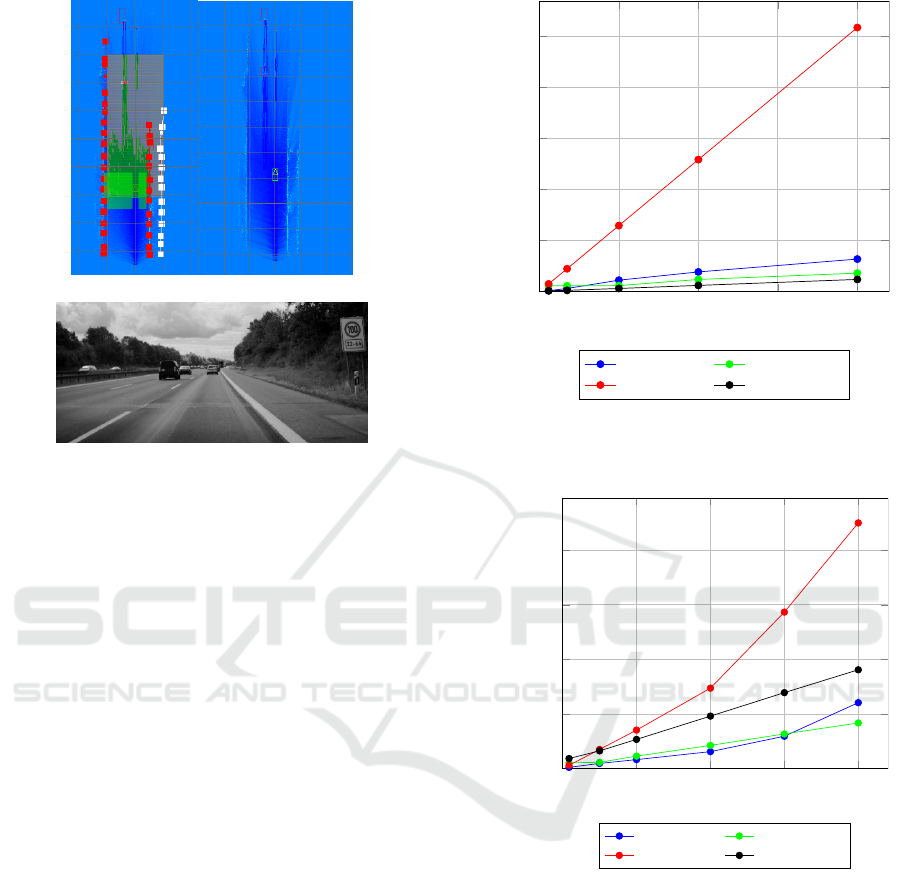
(a) (b)
(c)
Figure 4: One of the scenarios, that was used to test our
algorithm. (a) shows the grid map with annotations, like
dynamic and static objects. (b) shows the grid map without
notations. (c) shows the grayscale video image of the grid
maps in (a) and (b).
3 EVALUATION
3.1 Experimentation Platform
We used two platforms in our experiments. A desktop
PC, equipped with an Intel i7-3960X and an Nvidia
680 GTX GPU . The CPU has six cores with Hyper-
Threading and a maxiumum clock frequency of 3.9GHz .
The GPU on the desktop PC has 1536 CUDA cores and
1058MHz . As an embedded platform, an Nvidia Jetson
K1 board (NVIDIA Corp., 2016a) is used. It embodies
an ARM Cortex-A15 quad-core CPU with 2.3GHz
and a Tegra Kepler GPU with 192 CUDA cores, at
850MHz . This platform has typically only a power
consumption under workload of 8 − 10 W. So it can
be cooled passively, which is important for ECU s in
vehicles. Furthermore, the same GPU is also used by
the AUDI AG in their zFAS (Audi AG, 2016). We did
our experiments with real data, collected on a highway
by a car equipped with a laser scanner in the front of a
car. One of the driving scenarios is shown in Figure 4.
The laser scanner has a resolution of 581 channels in the
width and 3 layers in the height. For each experiment,
we averaged the measurements of 100 runs.
0
0.5
1
1.5
2
·10
4
0
5
10
15
20
25
laser beams
time in [ms]
CPU-Desktop GPU-Desktop
CPU-Jetson GPU-Jetson
Figure 5: Each single laser beam of the measurement is
transformed from polar to Cartesian space in homogeneous
coordinates.
0 2 4
6
8
·10
4
0
500
1,000
1,500
2,000
laser beams
time in [us]
CPU-Desktop GPU-Desktop
CPU-Jetson GPU-Jetson
Figure 6: Each single laser beam of the measurement is
compensated by the ego-motion of the own vehicle.
3.2 Experiments
3.2.1 Base Algorithms
One of the base algorithm, which is needed for creating
environment maps is the coordinate transformation from
polar to Cartesian coordinate space. For every laser
measurement, one CUDA thread was created on the
GPU . The results of that transformation, for different
sensor resolutions, are illustrated in Figure 5.
For a small number of laser beams, the CPU s on
both evaluation platforms are faster. The reason is
that the usage of a GPU always has a slight overhead,
Base Algorithms of Environment Maps and Efficient Occupancy Grid Mapping on Embedded GPUs
303

Table 1: Each single laser beam of the measurement is trans-
formed from polar to Cartesian space in homogeneous coordi-
nates on the Jetson K1 board. The results are in milliseconds
[ms].
Number of
laser channels K1-CPU K1-GPU
1743 min: 0.029
max: 0.662
avg.: 0.038
med.: 0.030
min: 0.024
max: 0.177
avg.: 0.093
med.: 0.092
10000 min: 0.171
max: 6.638
avg.: 0.287
med.: 0.175
min: 0.154
max: 0.348
avg.: 0.168
med.: 0.162
20000 min: 0.343
max: 8.011
avg.: 0.513
med.: 0.352
min: 0.257
max: 0.367
avg.: 0.271
med.: 0.267
40000 min: 0.690
max: 8.389
avg.: 1.116
med.: 0.736
min: 0.419
max: 0.613
avg.: 0.512
med.: 0.480
60000 min: 1.137
max: 11.973
avg.: 2.291
med.: 1.432
min: 0.628
max: 0.734
avg.: 0.693
med.: 0.695
80000 min: 1.876
max: 12.255
avg.: 3.513
med.: 2.248
min: 0.836
max: 0.939
avg.: 0.904
med.: 0.904
e.g., memory transfers or allocating of GPU memory.
Between 581 and 5000 laser beams, the execution time
on the desktop GPU is more or less the same. This is
due to the low utilization of the desktop GPU . There
are not enough calculations and memory transfers to
utilize this GPU rationally. The proportionally high
increase of the ARM-CPU on the Jetson board is due to
lesser special arithmetic units on the CPU, which can
calculate, the necessary trigonometric functions for the
coordinate transformation, in hardware.
In Table 1, measurement results of the coordinate
transformation with the minimum, maximum, average
and median values are given. The discrepancy between
the minimum and maximum value of one measurement
is on the CPU much higher than on the GPU . The
reason for that is, that on the CPU at the same time
interrupts of the operating system, without user input,
have to be handled. Instead, on the GPU , that is not the
case. The much more steady executions times on the
GPU are a further advantage, besides the speedup, be-
cause so the execution times are more predictable. The
high discrepancy was observed at all of the experiments.
In the next experiment, we evaluate the execution
times of the ego-motion compensation of the vehicle. As
Table 2: Average execution time of the coordinate transforma-
tion from polar to Cartesian space including bubble sort in ms
on the Nvidia Jetson K1 board.
Number of
laser channels ARM-
K1
K1-GPU Speedup
581 0.51 0.25 2.0
1162 0.93 0.26 3.5
2324 1.59 0.32 5.0
5810 4.14 0.57 7.3
described in Section 2, the single sensor measurements
can be directly compensated by the ego-motion of the
vehicle. Again, for each laser beam, a CUDA thread
was created. In Figure 6, the results of the experiments
are shown.
The break-even point, where the GPU is faster than
the CPU, is for the desktop computer by roundabout
60000 laser beams. For the Jetson K1 board, the break-
even point is instead already by roundabout 10000 laser
beams. The reason for the earlier break-even point on
the Jetson board is that the performance ration between
the desktop CPU and the desktop GPU is smaller than
on the embedded board, due to the high performance of
the desktop CPU. For a higher number of measurements
the speedup, between the GPU s and the CPU s versions
would further increase, in favor for the GPU s versions.
At a certain point, the speedup curve would flatten out,
if the GPU is fully utilized.
3.2.2 Novel Parallel Occupancy Grid Map
In Table 2, the results of the parallelization of the
coordinate transformation, including the bubble sort,
are shown. Only for every horizontal channel of the
laser scanner a CUDA thread was created, due to the
intrinsics of the bubble sort algorithm. The sorting of
the vertical layers of one horizontal channel is done
sequentially. A parallel sorting algorithm, like a bitonic
sorter (Batcher, 1968), was not rational usable, due
to the low number of vertical layers. The number
of vertical layers would have to be increased to an
unrealistic number ( > 1000 ), that this algorithm would
be efficient on a GPU . For every chosen resolution of
the laser, a speedup on the GPU could be achieved. The
speedups are only moderate because only for valid data
a coordinate transformation was done and in real-world
scenarios, which we used, quite a lot of data is not valid.
The higher the number of laser beams, the higher the
speedup is. The reason for this is that with a higher
number of laser beams, in the sum more arithmetic
operations and the GPU is better utilized.
Finally, the measurements have to be put into the
occupancy grid map. For that experiment, we paralleli-
VEHITS 2018 - 4th International Conference on Vehicle Technology and Intelligent Transport Systems
304

Table 3: Average execution time of the grid map update
including the determination of static an d dynamic objects in
ms on the Nvidia Jetson K1 board. For every channel (and not
additionally for every layer) a CUDA thread is started.
Number of
laser channels ARM-
K1
K1-GPU Speedup
581 1.51 1.79 0.8
1162 2.41 1.81 1.4
2324 4.13 1.78 5.0
5810 12.3 1.82 7.2
Table 4: Average execution time of the grid map update
including the determination of static an d dynamic objects in
ms on the Nvidia Jetson K1 board. For every channel and for
every layer a CUDA thread is started.
Number of
laser channels/
Number of
laser layers K1-
ARM
GPU-K1 Speedup
581/3 1.54 1.23 1.25
581/30 1.53 7.60 0.2
5810/3 11.96 4.92 2.43
5810/30 11.96 40.76 0.29
zed only the horizontal channels of the laser scanner.
The resolution of the laser scanner in the vertical di-
rection was always three. The results, therefore, are
shown in Table 3. The speedup increases with the
number of laser measurements, for the same reason
mentioned above. The execution time on the CPU
increases much more than on the GPU.
Since our laser scanner has not only laser beams in
the horizontal layer, but also in the vertical layer, we
created for every laser beam one thread. The result of
this parallelization is shown in Table 4.
For 581 laser beams in the horizontal layer, the
speedup was highe, than in the previous experiment,
where only the horizontal layers were parallelized. If
we increase the number of vertical layers, the GPU
version is slower than the CPU version. The reason
for that is our efficient algorithm. We have sorted the
vertical layers of one horizontal layer in the order of the
distance of the measurement. Only the measurement
of the shortest distance to an object is evaluated. This
means, a lot of threads are started on the GPU and then
have nothing to do, which creates an overhead.
4 CONCLUSION
In this paper, we demonstrated for several base algo-
rithms common in ADAS for automated driving, if
and for which sensor resolutions they can be efficiently
parallelized on a GPU . In almost all cases, the per-
formance on the GPU increased with an increasing
sensor resolution. The achieved speedups of the base
algorithms were higher than the whole update algorithm,
due to its less complex structure. Further, we presented,
a novel approach for the parallelization of an occupancy
grid map on a GPU . Therefore, we used the intrinsics
characteristics of the thread execution model by the
Nvidia framework CUDA and evaluated our approach
with real-time data collected on a highway.
REFERENCES
Audi AG (2016). Everything combined, all in one
place: The central driver assistance control
unit. http://www.audi.com/com/brand/en/
vorsprung_durch_technik/content/2014/10/
zentrales-fahrerassistenzsteuergeraet-zfas.
html.
Badino, H., Franke, U., Mester, R., and Main, F. A. (2007).
Free space computation using stochastic occupancy
grids and dynamic programming. In In Dynamic Vision
Workshop for ICCV.
Bar-Shalom, Y., Daum, F., and Huang, J. (2009). The proba-
bilistic data association filter. IEEE Control Systems,
29(6):82–100.
Batcher, K. E. (1968). Sorting networks and their applications.
In Proceedings of the Spring Joint Computer Conference
(AFIPS), AFIPS ’68 (Spring), pages 307–314, New York,
NY, USA. ACM.
Bresenham, J. E. (1965). Algorithm for computer control of a
digital plotter. IBM Systems Journal, 4(1):25–30.
Chen, C., Tay, C., Laugier, C., and Mekhnacha, K. (2006). Dy-
namic environment modeling with gridmap: A multiple-
object tracking application. In 2006 9th International
Conference on Control, Automation, Robotics and Vision,
pages 1–6.
Cover, T. and Hart, P. (2006). Nearest neighbor pattern
classification. IEEE Trans. Inf. Theor., 13(1):21–27.
Dryanovski, I., Morris, W., and Xiao, J. (2010). Multi-volume
occupancy grids: An efficient probabilistic 3d mapping
model for micro aerial vehicles. In Proceedings of
the IEEE/RSJ International Conference on Intelligent
Robots and Systems (IROS), pages 1553–1559.
Elfes, A. (1989). Using occupancy grids for mobile robot
perception and navigation. Computer, 22(6):46–57.
Fickenscher, J., Reiche, O., Schlumberger, J., Hannig, F.,
and Teich, J. (2016). Modeling, programming and
performance analysis of automotive environment map
representations on embedded GPUs. In 2016 IEEE
International High Level Design Validation and Test
Workshop (HLDVT), pages 70–77.
Base Algorithms of Environment Maps and Efficient Occupancy Grid Mapping on Embedded GPUs
305

Grisettiyz, G., Stachniss, C., and Burgard, W. (2005). Impro-
ving grid-based slam with Rao-Blackwellized particle
filters by adaptive proposals and selective resampling.
In Proceedings of the IEEE International Conference on
Robotics and Automation, pages 2432–2437.
Homm, F., Kaempchen, N., Ota, J., and Burschka, D. (2010).
Efficient occupancy grid computation on the GPU with
lidar and radar for road boundary detection. In Procee-
dings of the IEEE Intelligent Vehicles Symposium, pages
1006–1013.
Kalman, R. E. (1960). A new approach to linear filtering and
prediction problems. Transactions of the ASME–Journal
of Basic Engineering, 82(Series D):35–45.
Kammel, S. and Pitzer, B. (2008). Lidar-based lane marker
detection and mapping. In Proceedings of the IEEE
Intelligent Vehicles Symposium, pages 1137–1142.
Moravec, H. (1988). Sensor fusion in certainty grids for
mobile robots. AI Mag., 9(2):61–74.
Moravec, H. (1996). Robot spatial perception by stereoscopic
vision and 3d evidence grids. Technical Report CMU-
RI-TR-96-34, Carnegie Mellon University, Pittsburgh,
PA, USA.
Musicki, D. and Evans, R. (2004). Joint integrated proba-
bilistic data association: Jipda. IEEE Transactions on
Aerospace and Electronic Systems, 40(3):1093–1099.
NVIDIA Corp. (2016a). NVIDIA Jetson TK1 De-
veloper Kit. http://www.nvidia.com/object/
jetson-tk1-embedded-dev-kit.html.
NVIDIA Corp. (2016b). Programming guide – CUDA toolkit
documentation. https://docs.nvidia.com/cuda/
cuda-c-programming-guide/.
Sebastian Thrun, Wolfram Burgard, D. F. (2005). Probalistic
Robotics. The MIT Press, Cambridge, Massachusetts
and London, England.
Werber, K., Rapp, M., Klappstein, J., Hahn, M., Dickmann, J.,
Dietmayer, K., and Waldschmidt, C. (2015). Automotive
radar gridmap representations. In 2015 IEEE MTT-S
International Conference on Microwaves for Intelligent
Mobility (ICMIM), pages 1–4.
Yguel, M., Aycard, O., and Laugier, C. (2006). Efficient
gpu-based construction of occupancy girds using several
laser range-finders. In Intelligent Robots and Systems,
2006 IEEE/RSJ International Conference on, pages
105–110.
VEHITS 2018 - 4th International Conference on Vehicle Technology and Intelligent Transport Systems
306