Approximate Epipolar Geometry from Six Rotation Invariant

Correspondences

aniel Bar

ath

MTA SZTAKI, Kende u. 13-17, Budapest H-1111, Hungary

ELTE IK, P

azm

any P

eter s

any 1/C, H-1117 Budapest, Hungary

Keywords:

Fundamental Matrix, Epipolar Geometry, Rotation Invariant Features, Approximation.

Abstract:

We propose a method for estimating an approximate fundamental matrix from six rotation invariant feature

correspondences exploiting their rotation components, e.g. provided by SIFT or ORB detectors. The cameras

are not calibrated. First, a linear sub-space is calculated from the point coordinates, then the rotations are used

assuming orthographic projection. It is demonstrated that combining the proposed method with Graph-cut

RANSAC makes it superior to the state-of-the-art in terms of accuracy for tasks requiring a strict time limit.

These tasks are practically the ones which need to be done real time. We tested the method on 203 publicly

available real image pairs.

1 INTRODUCTION

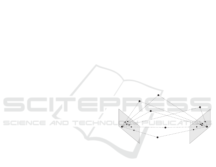
In this paper, we aim to approximate the epipolar ge-

ometry between two non-calibrated cameras exploi-

ting six rotation invariant feature correspondences in

general position (see Fig. 1). The approximated fun-

damental matrix F ∈ R

3×3

is then used in a recent

variant of locally optimized RANSAC (Chum et al.,

2003) making it faster than the state-of-the-art due

to the reduced number of the required points. This

speedup is beneﬁcial in online applications, i.e. when

real time processing is needed, and leads to results

superior to the state-of-the-art in terms of accuracy.

The common techniques to estimate the funda-

mental matrix when no camera parameters are known,

i.e. the non-calibrated case, are the eight- and seven-

point methods (Hartley and Zisserman, 2003). Both

of them are widely-used in computer vision applicati-

ons and have thousands of citations year-by-year. The

eight-point algorithm is based on estimating the direct

linear transformation which the epipolar constraint in-

duces. The method is fast and the stability issues had

already been solved by the normalization technique of

Hartley (Hartley, 1997) making the technique accu-

rate despite the noise. The seven-point algorithm en-

forces the rank-two constraint, i.e. the determinant of

F must be zero, by solving the cubic polynomial equa-

tion which it implies.

Getting more information using exclusively point

correspondences is not possible. Nevertheless, se-

Figure 1: The projections on cameras C

and C

of six 3D

points P

(i ∈[1,6]) in general position.

veral approaches had been proposed to reduce the

number of unknowns. As an example, knowing

the intrinsic parameters of the cameras (focal length,

pixel ratio or the principal point) makes the so-called

trace constraint applicable. The problem becomes

solvable using six (Li, 2006; Kukelova et al., 2008;

Stew

enius et al., 2008; Torii et al., 2010) correspon-

dences in the semi-calibrated case – when all intrinsic

parameters are known but a common focal length. For

fully calibrated cameras, ﬁve (Nist

er, 2004; Li and

Hartley, 2006; Batra et al., ; Kukelova et al., 2008;

Hartley and Li, 2012) point pairs are enough for esti-

mating the relative motion. One can also restrict the

camera movement, e.g. the one point method propo-

sed by Davide Scaramuzza (Scaramuzza, 2011) assu-

mes the cameras to move on a plane and the so-called

non-holonomic constraint to hold.

464

Baráth, D.

Approximate Epipolar Geometry from Six Rotation Invariant Correspondences.

DOI: 10.5220/0006678304640471

In Proceedings of the 13th International Joint Conference on Computer Vision, Imaging and Computer Graphics Theory and Applications (VISIGRAPP 2018) - Volume 5: VISAPP, pages

464-471

ISBN: 978-989-758-290-5

Approaching the problem from a different di-

rection, it is very rare nowadays to have solely the

point coordinates obtained by the feature detector. For

example, SIFT (Lowe, 1999) features contain a rota-

tion and a scale or ORB (Rublee et al., 2011) features

provide a rotation. This plus information is usually

not used in recent geometric model estimators. It is

just thrown away at the very beginning. In this paper,

we involve an additional afﬁne parameter, i.e. rotation

of the feature, into the fundamental matrix estimation

process to reduce the size of the minimal sample re-

quired for fundamental matrix estimation.

Of course, using full afﬁne correspondences

(point pair together with rotation, shear and scales

along the image axes) for epipolar geometry estima-

tion is not a new idea. Perdoch et al. (Perdoch et al.,

2006) proposed techniques for approximating the es-

sential and fundamental matrix exploiting two and

three correspondences, respectively. Barath et al. (Ba-

rath et al., 2017) showed that using two afﬁne corre-

spondences, the fundamental matrix and a common

focal length can be estimated simultaneously. Raposo

et al. (Raposo and Barreto, 2016) proposed a solution

for essential matrix estimation using two correspon-

dences. Bentolila et al. (Bentolila and Francos, 2014)

proposed a method to estimate the F from three cor-

respondences proposing conic constraints.

Exploiting only a part of an afﬁne correspondence,

e.g. exclusively the rotation component, is a well-

known technique for example in wide-baseline fea-

ture matching (Matas et al., 2004). To the best of our

knowledge, the sole work involving them into geo-

metric model estimation is (Barath, 2017). It assu-

mes that F is known a priori and a technique is pro-

posed for estimating a homography using two SIFT

correspondences using their scale and rotation com-

ponents. Nevertheless, they consider that the scales

along axes u and v equal to that of the SIFT features –

which is practically not true. Thus the method obtains

an approximation of the homography.

The contributions of this paper: (i) the relations-

hip of afﬁne correspondences and epipolar geometry

proposed in (Barath et al., 2017) are reformulated ma-

king it separable to orientation and scale components.

(ii) Using the proposed formulas, we assume that the

orientation constraint can be satisﬁed by the rotation

of the feature, thus making the fundamental matrix

estimable from six correspondences. It is demonstra-

ted on 203 real image pairs that the proposed method

combined with a recent variant of locally optimized

RANSAC outperforms the state-of-the-art if real time

performance is required.

2 THEORETICAL BACKGROUND

Afﬁne Correspondences. In this paper, we con-

sider an afﬁne correspondence (AC) as a triplet:

,A), where p

= [u

and p

are a corresponding homogeneous point

pair in the two images, and

A =





is a 2 ×2 linear transformation which we call local

afﬁne transformation. To deﬁne A, we use the deﬁ-

nition provided in (Moln

ar and Chetverikov, 2014) as

it is given as the ﬁrst-order Taylor-approximation of

the 3D → 2D projection functions. Note that, for per-

spective cameras, A is the ﬁrst-order approximation

of the related homography matrix

H =









as follows:

∂u

−h

, a

∂u

∂v

−h

∂v

∂u

−h

, a

∂v

−h

(1)

where u

and v

are the directions in the ith image

(i ∈{1,2}) and s = u

+ v

+ h

is the projective

depth.

Fundamental Matrix

F =









is a 3×3 transformation matrix ensuring the so-called

epipolar constraint p

= 0 for rigid scenes. Since

its scale is arbitrary and det(F) = 0, F has seven

degrees-of-freedom (DoF).

The relationship of afﬁne correspondences and

epipolar geometry is deﬁned in (Barath et al., 2017)

as follows:

−T

)

(1:2)

= (Fp

)

(1:2)

, (2)

where operator v

(i: j)

selects a sub-vector consisting of

the elements of vector v from the ith to the jth. Vector

is basically the normal of the epipolar line on

which point p

lies in the ﬁrst image, and Fp

is the

same for p

. Expanding this formula leads to a system

of two linear, homogeneous equations as follows:

+ a

) f

+ a

+ (v

+ a

) f

+ a

+ f

= 0, (3)

+ (u

+ a

) f

+ a

) f

+ a

+ f

= 0. (4)

Approximate Epipolar Geometry from Six Rotation Invariant Correspondences

465

Thus each afﬁne correspondence reduces the degrees-

of-freedom by three. Having three of them are enough

for the estimation. These properties will help us to

recover an approximate fundamental matrix from six

rotation invariant feature correspondences.

3 FUNDAMENTAL MATRIX

ESTIMATION

In this section, we ﬁrst propose two constraints refor-

mulating the one given in (Barath et al., 2017). Com-

paring to the original one, the proposed constraints are

separable into two, geometrically interpretable (rota-

tion and scaling), transformations. We simplify the

afﬁne transformation model using the given rotations

and this simpliﬁed model is then used to approximate

the fundamental matrix.

3.1 Geometric Constraints

As it was shown before, an afﬁne correspondence

yields three linear equations. However, in our case,

not a full afﬁne correspondence is given but a part

of it: the point coordinates and a rotation. There-

fore, assume point pair p

, p

and the related angle,

α ∈ [0,2π), to be known in two images.

To exploit solely the rotation from the local afﬁne

transformation Eqs. 2 have to be reformulated. First

replace F

and Fp

by the related normals as

−T

= −n

It means that the coordinates of the line normal in the

ﬁrst image n

= [n

u,1

v,1

]

must be mapped to its

coordinates n

= [n

u,2

v,2

]

in the second one by

−T

. This relationship can be separated into orienta-

tion and scale components.

The orientation constraint states that A

−T

must

rotate the direction of n

into that of n

as follows:

−T

k n

This can be written as

−T

)

|An

||n

= cos(0) = 1.

In order to eliminate the length calculation (|A

−T

and |n

|), it is beneﬁcial to require perpendicularity

instead of parallelity. Thus the original equations are

formulated equivalently in the following way:

−T

)

π/2

|An

||R

π/2

= cos(π/2) = 0, (5)

where R

π/2

is an orthonormal 2D rotation matrix rota-

ting by π/2 radians and R

π/2

(= v

= [v

u,2

v,2

]

)

is basically the tangent direction of the epipolar line

in the second image. R

π/2

is as follows:

π/2



cos(

) −sin(

)

sin(

) cos(

)





0 −1

1 0



Since for requiring Eq. 5 to be zero, the lengths do not

have to be estimated. Thus Eq. 5 becomes

−T

)

π/2

= 0.

To avoid inversion this can be written as follows:

π/2

)

) = 0.

This formula leads to the following equation

u,2

+ a

v,2

u,1

+ (a

u,2

+ a

v,2

v,1

= 0.

Remember that n

and v

are computed from the fun-

damental matrix. They are as

= R

π/2

= R

π/2

)

(1:2)

π/2



+ f





+ f

−f

− f



and

= (Fp

)

(1:2)



+ f



The ﬁnal formula encapsulating the orientation con-

straint is the following:

(−u

−v

− f

)(a

+ v

+ f

+ v

+ f

)(a

+ v

+ f

+ v

+ f

)) + a

+ v

+ f

)) = 0

(6)

The scale constraint states that the length of the

transformed normal in the ﬁrst image must be the in-

verse of that in the second one. Due to A

−T

= −n

| equals to |A

|. Therefore,

u,1

+ n

v,1

= (a

u,2

+ a

v,2

)

+ (a

u,2

+ a

v,2

)

(7)

The ﬁnal formula for the scale constraint (after re-

arranging Eq. 7 and substituting the elements of the

fundamental matrix) is as follows:

( f

+ f

)

+ ( f

+ f

)

−

( f

+ f

) + a

( f

+ f

))

−

( f

+ f

) + a

( f

+ f

))

= 0

(8)

3.2 Fundamental Matrix Estimation

Suppose that six point pairs p

1,i

= [u

1,i

2,i

= [u

2,i

, (i ∈ [1,6]) in their homogene-

ous form and the corresponding rotations α

are gi-

ven. The task is to estimate fundamental matrix F

which is compatible with both the point coordina-

tes and the given rotations. In order to reduce the

VISAPP 2018 - International Conference on Computer Vision Theory and Applications

466

number of unknowns we ﬁrst form a linear homoge-

neous equation system Cx = 0 from the point coor-

dinates via the well-known formula, p

2,i

1,i

= 0.

Vector x = [ f

]

consists of the unknown variables and coefﬁcient ma-

trix C ∈ R

6×9

is as follows:

C =





1,1

2,1

1,1

2,1

1,1

2,1

1,1

2,1

1,1

...

1,6

2,6

1,6

2,6

1,6

2,6

1,6

2,6

1,6





Since the null-space of C is three-dimensional, F can

be calculated as their linear combination as

F = βe + γg + δh, (9)

where β, γ and δ are unknown scalars, e = [e

... e

]

g = [g

... g

]

and h = [h

... h

]

are the null-vectors.

Due to the scale ambiguity of F one scale can be cho-

sen to an arbitrary value, thus δ = 1 in our algorithm.

In order to exploit the given rotations we approx-

imate the afﬁne transformation model assuming that

the orientation constraint (Eq. 8) can be satisﬁed by

purely a rotation. Note that, without proof, this as-

sumption holds for orthogonal projection. However,

for perspective projection, the shear also affects Eq. 8.

This approximation means that A

≈ R

, where R

is a 2D rotation matrix rotating by α

radians. We do

not exploit the scale constraint, since no information

is available about how A scales the normal of the re-

lated epipolar line.

Replacing each f

with βe

+ γg

+ h

Eq. 8 leads to a multivariate polynomial equa-

tion (see Appendix 5 for details) with monomials

[β

βγ β γ 1]

. Since we are given

six rotations, it yields six polynomial equations.

Considering each monomial as an independent

variable the obtained inhomogeneous linear system

Dh = d becomes solvable, where D is the coefﬁcient

matrix, h = [β

βγ β γ]

consists of the

unknown variables and d is the vector containing

the inhomogeneous part of the equations. The ﬁnal

solution is obtained as h = D

†

d, where D

†

is the

Moore-Penrose pseudo-inverse of matrix D. The

ﬁnal fundamental matrix is calculated by substituting

the obtained β and γ into Eq. 9. Note that it is

beneﬁcial to get the ﬁnal scalars as β =

√

and

γ =

√

. Due to the approximation we made, F

is not the exact fundamental matrix. However, it is

good starting point for numerical optimization or, as

we will demonstrate it later, for locally optimized

robust estimators like LO-RANSAC (Chum et al.,

2003).

Robustness: is achieved by normalizing the coefﬁ-

cients of each polynomial equation making their sum

one. It is also beneﬁcial to apply the normalization

technique of Hartley (Hartley, 1997) which is as fol-

lows: given a set {(p

1, j

2, j

)}

j=1

of n point corre-

spondences in their homogeneous forms. Normali-

zing transformation T

in the ith image (i ∈ {1,2}) is

as follows:





√

2/d

0 0

√

2/d

0 0 1









1 0 −¯u

0 1 −¯v

0 0 1





where

= [ ¯u

, ¯v

,1]

is the mean of the point set in

the ith image and

∑

j=1

−

p) (10)

is its average distance from the mean. Applying

the normalizing transformations, the normalized cor-

respondence set is as follows: {(

1, j

2, j

)}

j=1

{(T

1, j

2, j

)}

j=1

. After the estimation, F is cal-

culated from the normalized fundamental matrix

as follows: F = T

−T

−1

. Note that the normali-

zing transformations consist of a scale and a transla-

tion, therefore, the rotations of the features remain the

same, they do not have to be modiﬁed.

3.3 Processing Time

The proposed method consists of two main steps: (i)

the null-space computation of a matrix of size 6 ×9.

(ii) Using the estimated null-vectors and the rotation

components, a coefﬁcient matrix of size 6 ×5 is built

and its null-space is computed. The average proces-

sing time of 100 runs of our C++ implementation

using OpenCV was 0.03 milliseconds.

Combining hypothesize-and-verify robust estima-

tors, like RANSAC (Fischler and Bolles, 1981), with

the proposed method is beneﬁcial since their proces-

sing time highly depends on the size of the minimal

sample required for the estimation. Table 1 shows

the theoretically needed iteration number of RAN-

SAC combined with minimal methods (columns) on

different outlier levels (rows). The conﬁdence value

was set to 95%. It can be seen that using the proposed

6-point algorithm leads to signiﬁcant improvement in

the processing time.

4 EXPERIMENTAL RESULTS

In this section, we will compare the proposed method

with the eight- and seven-point algorithms on publicly

available real datasets.

Approximate Epipolar Geometry from Six Rotation Invariant Correspondences

467

Table 1: Required theoretical iteration number of RAN-

SAC (Fischler and Bolles, 1981) combined with minimal

methods (columns) with conﬁdence set to 95% on different

outlier levels (rows).

Conﬁdence 95%

Outl. 6 7 8

50% 190 382 765

80% ∼ 10

∼ 10

95% ∼ 10

∼ 10

99% ∼ 10

∼ 10

In order to overcame the approximative nature of

the proposed approximating six-point technique we

combined it with a recent variant of locally optimized

RANSAC (Chum et al., 2003). We chose Graph-Cut

RANSAC (Barath and Matas, 2017) (GC-RANSAC)

as robust estimator since it can be considered as state-

of-the-art and its source code is publicly available

Brieﬂy, it replaces the local optimization step of LO-

RANSAC with graph-cut applied to the current best

model. In the local optimization step, we used the

normalized eight-point algorithm. Thus the approxi-

mated fundamental matrix is used only as an initial es-

timate to determine a set of inliers, then the obtained F

is reﬁned iteratively exploiting a set of corresponden-

ces, i.e. the inliers. We used the same parameters as

the authors proposed: the inlier-outlier threshold was

set to 0.31, the iteration limit to 5000 and the weight

of the spatial coherence term was 0.14.

We used the AdelaideRMF, Kusvod2, Multi-H,

and Strecha datasets (see Fig. 2) to evaluate the propo-

sed method on real world data. AdelaideRMF, Kus-

vod2 and Multi-H contains image pairs of size from

455 × 341 to 2592 ×1944 and manually annotated

point correspondences (assigned to the outlier or in-

lier classes) for each pair. Since the reference points

do not contain rotation components we detected and

matched points applying ORB feature detector (Ru-

blee et al., 2011). ORB features contain the orienta-

tion and the point coordinates.

Strecha dataset contains image sequences toget-

her with projection matrices. Each image is of resolu-

tion 3072 ×2048. The fundamental matrices are esti-

mated for all possible image pairs in every sequence.

Correspondences were obtained by ORB detector and

the ground truth fundamental matrices were calcula-

ted from the given projection matrices (Hartley and

Zisserman, 2003). All detected point pairs were con-

sidered as reference points for which the symmetric

epipolar distance (Hartley and Zisserman, 2003) from

the ground truth F was smaller than 1.0 pixels. To dis-

card not stable image pairs, the minimum reference

point number was set to 10. Thus every image pair

https://github.com/danini/graph-cut-ransac

for which less than 10 correspondences were closer

to the ground truth F than one pixels was not used in

the evaluation.

We used the reference point sets to validate the

estimated fundamental matrices. The reported geo-

metric errors were computed as the mean symmetric

epipolar distance as

∑

)∈P

(Fp

)

+ (Fp

)

+ (p

(11)

where P

is the set consisting of the reference point

correspondences.

The competitor methods, i.e. the minimal sol-

vers combined with GC-RANSAC, were the normali-

zed eight- and seven-point algorithms

. In the least-

squares model re-ﬁtting step of GC-RANSAC, the

normalized eight-point method was applied using the

current inlier set.

Table 3 reports the mean result of 100 runs on

every pair from the Strecha dataset. The ﬁrst column

denotes the name of the sequence, the second one is

the number of the image pairs used – the ones for

which more than 10 reference points were kept. The

next two blocks, each consisting of three columns,

shows the results of the methods if the conﬁdence

of GC-RANSAC is set to 99% (ﬁrst block) and for a

strict time limit (60 FPS; second block). The reported

properties are the mean and median geometric errors

of the estimated fundamental matrices (Eq. 11) w.r.t.

the reference point sets, and the number of the sam-

ples, i.e. iterations, drawn by GC-RANSAC. It can

be seen that for no time limit (ﬁrst three columns),

the seven-point algorithm obtains the most accurate

results on average. This is not surprising since it is

a consistent estimator (for no noise the error is zero)

and “iniﬁte” time is given to get the most accurate re-

sult. It can also be seen that if there is a strict time

limit to achieve real time performance (last three co-

lumns), the proposed method yields the most accurate

results.

Table 2 shows the mean results on AdelaideRMF,

Kusvod2 and Multi-H datasets (ﬁrst column) if the

conﬁdence is set to 99% (third – sixth column). The

last three columns report the results if there is a strict

60 frames-per-seconds (FPS) time limit. The same

property can be seen as for the Strecha dataset: (i) for

no time limit, the best is the seven-point algorithm.

(ii) For 1/60 FPS, the proposed approximating six-

point method combined with GC-RANSAC leads to

the most accurate fundamental matrix estimates.

The implementation provided in OpenCV is used for

the eight- and seven-point algorithms.

VISAPP 2018 - International Conference on Computer Vision Theory and Applications

468

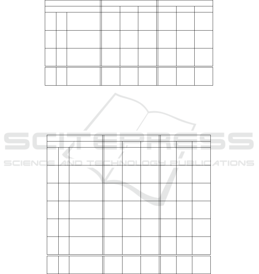
Table 2: Fundamental matrix estimation on the (a) Kusvod2, (b) AdelaideRMF, and (c) Multi-H datasets applying GC-

RANSAC (Barath and Matas, 2017) combined with minimal methods (second row). The number of the image pairs and the

properties are written into the second and third columns. The results at 99% conﬁdence are reported in the next three. The last

three columns contain the results for a time limit set to 60 FPS, i.e. the run is interrupted after 1/60 secs. Values are computed

as the means of 100 runs on each test pair. The mean and median errors (in pixels) of the estimated model w.r.t. the manually

annotated inliers are written in each ﬁrst and second rows; the required number of samples are reported in every third row.

Conﬁdence 99% 60 FPS

Minimal methods 6 7 8 6 7 8

(a)

Avg Err (px) 21.67 23.78 47.67 16.62 20.18 45.38

Med Err (px) 22.45 24.72 43.50 13.88 21.81 44.06

Samples 4992 5000 5000 74 119 380

(b)

Avg Err (px) 4.63 3.04 6.72 4.00 3.67 7.63

Med Err (px) 3.63 2.33 4.05 3.56 2.82 4.87

Samples 4982 5000 5000 74 136 292

(c)

Avg Err (px) 4.17 4.45 11.26 4.52 4.59 12.18

Med Err (px) 4.46 4.91 11.41 4.15 4.54 11.55

Samples 5000 5000 5000 51 83 403

(all)

Avg Err (px) 13.48 13.98 28.48 10.63 12.36 27.72

Med Err (px) 10.18 10.65 19.65 7.20 9.72 20.16

Samples 5000 5000 5000 72 122 349

Table 3: Fundamental matrix estimation on the Strecha dataset applying GC-RANSAC (Barath and Matas, 2017) combined

with minimal methods (second row). The ﬁrst column contains the names of the sequences: (a) fountain-p11, (b) entry-p10,

(c) castle-p19, (d) castle-p30, (e) herzjesus-p8, and (f) herzjesus-p25. The number of the image pairs and the properties are

written into the second and third columns. The results at 99% conﬁdence are reported in the next three. The last three columns

contain the results for a time limit set to 60 FPS, i.e. the run is interrupted after 1/60 secs. Values are computed as the means

of 100 runs on each test pair. The mean and median errors (in pixels) of the estimated model w.r.t. the manually annotated

inliers are written in each ﬁrst and second rows; the required number of samples are reported in every third row.

Conﬁdence 99% 60 FPS

Minimal methods 6 7 8 6 7 8

(a)

Avg Err (px) 1.93 9.75 7.19 1.84 5.71 6.26

Med Err (px) 0.99 3.42 2.78 0.98 1.64 3.12

Samples 4 394 5 748 5 721 279 352 447

(b)

Avg Err (px) 30.15 7.83 13.67 5.71 7.04 41.90

Med Err (px) 4.64 1.74 3.08 1.56 2.27 39.71

Samples 4 981 5 121 5 004 134 183 284

(c)

Avg Err (px) 2.43 3.98 12.62 5.42 7.16 20.00

Med Err (px) 1.77 2.90 4.62 1.69 5.46 9.87

Samples 4 575 5 355 5 613 210 348 436

(d)

Avg Err (px) 9.24 5.11 10.73 3.33 6.29 9.82

Med Err (px) 2.92 1.89 4.24 1.32 2.11 4.49

Samples 5 669 6 306 6 339 200 311 392

(e)

Avg Err (px) 2.34 1.77 16.51 2.85 3.11 8.50

Med Err (px) 0.81 1.50 4.75 2.05 1.73 2.65

Samples 6 492 6 708 6 757 199 249 382

(f)

Avg Err (px) 5.47 4.31 10.50 1.24 2.27 6.46

Med Err (px) 1.71 1.84 2.57 1.24 1.32 2.71

Samples 6 305 6 708 6 758 179 240 361

(all)

157

Avg Err (px) 6.33 5.04 11.17 3.62 4.80 12.95

Med Err (px) 1.93 1.87 3.49 1.36 2.11 3.96

Samples 5 613 6 199 6 252 200 280 387

Fig. 2 shows example image pairs from each da-

taset with the epipolar lines of 50 random inliers. It

can be seen, that the results seem good: the epipolar

lines go through the same pixels in the ﬁrst (left) and

second (right) images.

5 CONCLUSION

In this paper, we proposed a method for approx-

imating the fundamental matrix between two non-

calibrated views from six rotation invariant feature

Approximate Epipolar Geometry from Six Rotation Invariant Correspondences

469

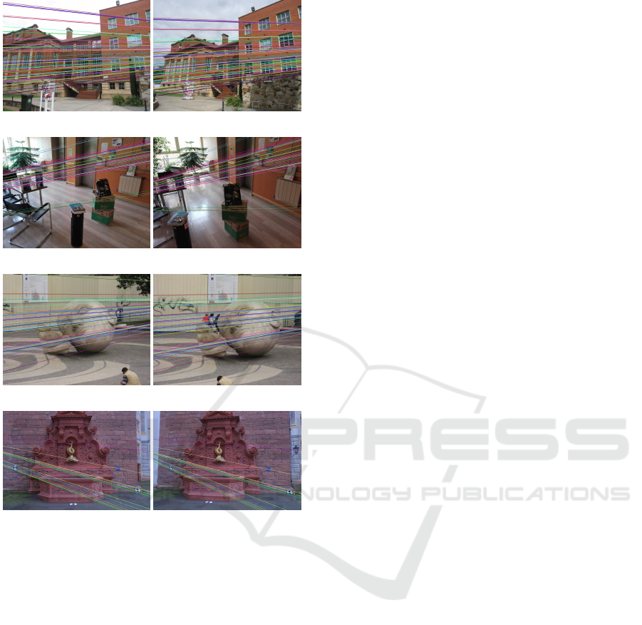
(a) AdelaideRMF

(b) Multi-H

(d) Strecha

Figure 2: The results of the proposed method combined

with Graph-Cut RANSAC. An image pair from each dataset

with the corresponding epipolar lines of 50 random inliers

drawn by colors.

correspondences. The method is solved through the

null-space computation of two matrices of sizes 6×9

and 6 ×5, thus achieving fast calculation, i.e. around

0.03 milliseconds in C++. Due to the reduced number

of required samples, the approximating six-point al-

gorithm combined with locally optimized RANSAC

obtains results superior to the state-of-the-art if a strict

time limit is given.

ACKNOWLEDGEMENTS

This research was supported by the Hungarian Scien-

tiﬁc Research Fund (No. OTKA/NKFIH 120499),

the Hungarian National Research, Development and

Innovation Ofﬁce under the grant VKSZ 14-1-2015-

0072, and the European Union, co-ﬁnanced by

the European Social Fund (EFOP-3.6.3-VEKOP-16-

2017-00001).

REFERENCES

Barath, D. (2017). P-HAF: Homography estimation using

partial local afﬁne frames. In VISAPP.

Barath, D. and Matas, J. (2017). Graph-cut ransac. ArXiv

preprint arXiv:1706.00984.

Barath, D., Toth, T., and Hajder, L. (2017). A minimal so-

lution for two-view focal-length estimation using two

afﬁne correspondences. In Conference on Computer

Vision and Pattern Recognition.

Batra, D., Nabbe, B., and Hebert, M. An alternative formu-

lation for ﬁve point relative pose problem. In Works-

hop onMotion and Video Computing.

Bentolila, J. and Francos, J. M. (2014). Conic epipolar con-

straints from afﬁne correspondences. Computer Vision

and Image Understanding.

Chum, O., Matas, J., and Kittler, J. (2003). Locally optimi-

zed ransac. In Joint Pattern Recognition Symposium.

Fischler, M. A. and Bolles, R. C. (1981). Random sample

consensus: a paradigm for model ﬁtting with appli-

cations to image analysis and automated cartography.

Communications of the ACM.

Hartley, R. and Li, H. (2012). An efﬁcient hidden variable

approach to minimal-case camera motion estimation.

Pattern Analysis and Machine Intelligence.

Hartley, R. and Zisserman, A. (2003). Multiple view geome-

try in computer vision. Cambridge University Press.

Hartley, R. I. (1997). In defense of the eight-point algo-

rithm. Pattern Analysis and Machine Intelligence.

Kukelova, Z., Bujnak, M., and Pajdla, T. (2008). Polyno-

mial eigenvalue solutions to the 5-pt and 6-pt relative

pose problems. In British Machine Vision Conference.

Li, H. (2006). A simple solution to the six-point two-view

focal-length problem. In European Conference on

Computer Vision.

Li, H. and Hartley, R. (2006). Five-point motion estimation

made easy. In International Conference on Pattern

Recognition.

Lowe, D. G. (1999). Object recognition from local scale-

invariant features. In International Conference on

Computer vision.

Matas, J., Chum, O., Urban, M., and Pajdla, T. (2004). Ro-

bust wide-baseline stereo from maximally stable ex-

tremal regions. Image and vision computing.

Moln

ar, J. and Chetverikov, D. (2014). Quadratic transfor-

mation for planar mapping of implicit surfaces. Jour-

nal of Mathematical Imaging and Vision.

Nist

er, D. (2004). An efﬁcient solution to the ﬁve-point

relative pose problem. Pattern Analysis and Machine

Intelligence.

Perdoch, M., Matas, J., and Chum, O. (2006). Epipolar

geometry from two correspondences. In International

Conference on Pattern Recognition.

Raposo, C. and Barreto, J. P. (2016). Theory and practice

of structure-from-motion using afﬁne corresponden-

ces. In Computer Vision and Pattern Recognition.

VISAPP 2018 - International Conference on Computer Vision Theory and Applications

470

Rublee, E., Rabaud, V., Konolige, K., and Bradski, G.

(2011). ORB: An efﬁcient alternative to sift or surf.

In Computer Vision (ICCV), 2011 IEEE international

conference on, pages 2564–2571. IEEE.

Scaramuzza, D. (2011). 1-point-ransac structure from mo-

tion for vehicle-mounted cameras by exploiting non-

holonomic constraints. International Journal of Com-

puter Vision.

Stew

enius, H., Nist

er, D., Kahl, F., and Schaffalitzky, F.

(2008). A minimal solution for relative pose with

unknown focal length. Image Vision Computing.

Torii, A., Kukelova, Z., Bujnak, M., and Pajdla, T. (2010).

The six point algorithm revisited. In Asian Conference

on Computer Vision.

APPENDIX

Formulas for the Orientation Constraint

Replacing each f

with βe

+ γg

+ h

in Eq. 8 leads to

a multivariate polynomial equation with monomials

[β

βγ β γ 1]

. The coefﬁcients regarding

to each monomial are shown in Figure 3.

: −a

+ a

−a

+ a

−a

+ a

−a

+ a

−a

+ a

−a

+ a

−a

+ a

−a

+ a

−a

+ a

−a

+ a

−a

−

+ a

−a

+ a

: −a

+ a

−a

+ a

−a

+ a

−a

+ a

−a

+ a

−a

+ a

−a

+ a

−a

+ a

−a

+ a

−a

+ a

−a

+ a

−a

+ a

βγ : −2a

+ a

−a

+ a

−a

+ a

−a

−

+ 2a

+ a

−a

+ a

−a

+ a

−a

+ a

−a

+ a

−a

+ a

−a

−2a

+ a

−a

+ a

−a

+ a

−a

+ a

−a

+ a

−a

+ 2a

−a

+ a

−a

+ a

−a

+ a

−

+ a

−a

+ a

−a

+ a

−a

+ a

−a

+ a

β : −2a

+ a

−a

+ a

−a

+ a

−a

−

+ 2a

+ a

−a

+ a

−a

+ a

−a

+ a

−a

+ a

−a

+ a

−a

−2a

−a

+ a

−a

+ a

−a

+ a

−a

+ a

−a

+ 2a

−a

+ a

−a

+ a

−a

+ a

−a

+ a

−

+ a

−a

+ a

−a

+ a

−a

+ a

γ : −2a

+ a

−a

+ a

−a

+ a

−a

−

+ 2a

+ a

−a

+ a

−a

+ a

−a

+ a

−a

+ a

−a

+ a

−a

−2a

+ a

−a

+ a

−a

+ a

−a

+ a

−a

+ a

−a

+ 2a

−a

+ a

−a

+ a

−a

+ a

−a

+ a

−a

+ a

−a

+ a

−a

+ a

1 : −a

+ a

−a

+ a

−a

+ a

−a

+ a

−a

+ a

−a

+ a

−a

+ a

−a

+ a

−a

+ a

−a

+ a

−a

+ a

−a

−

+ a

−a

+ a

Figure 3: The coefﬁcient for each monomial in the polynomial equation to which the orientation constraint lead (Eq. 8).

Approximate Epipolar Geometry from Six Rotation Invariant Correspondences

471