
Performance and Energy-based Cost Prediction of Virtual Machines
Live Migration in Clouds
Moahammad Aldossary
1,2
and Karim Djemame
2
1
Prince Sattam Bin Abdulaziz University, K.S.A.
2
School of Computing, University of Leeds, Leeds, U.K.
Keywords: Cloud Computing, Cost Prediction, Workload Prediction, Live Migration, Power Consumption.
Abstract: Virtual Machines (VMs) live migration is one of the important approaches to improve resource utilisation and
support energy efficiency in Clouds. However, VMs live migration leads to performance loss and additional
costs due to increased migration time and energy overhead. This paper introduces a Performance and Energy-
based Cost Prediction Framework to estimate the total cost of VMs live migration by considering the resource
usage and power consumption, while maintaining the expected level of performance. A series of experiments
conducted on a Cloud testbed show that this framework is capable of predicting the workload, power
consumption and total cost for heterogeneous VMs before and after live migration, with the possibility of
recovering the migration cost e.g. 28.48% for the predicted cost recovery of the VM.
1 INTRODUCTION
With the increasing cost of electricity, cloud
providers consider energy consumption as one of the
biggest operational cost factors to be managed within
their infrastructures. Most of the existing studies have
focused on minimising the energy consumption and
maximising the total resource usage, instead of
improving the performance. Further, cloud providers
such as Amazon
1
, have established their Service
Level Agreements (SLAs) based on service
availability without such an assurance of the
performance. For instance, during service operation,
when the number of VMs increases on the same
Physical Machine (PM) stretching its capacity to its
limits, resource competition may occur (e.g. once the
workload exceeds the acceptable level of CPU such
as 85% threshold) leading to VMs performance
degradation which may affect the fulfilment of the
SLAs and hence the cloud provider’s revenue. Hence
to prevent such performance loss effects, it is
necessary to have preventive actions such as re-
allocating and migrating VMs.
VMs live migration is an important mechanism to
improve resource utilisation and achieve energy
efficiency in Clouds. Live migration allows VMs to
1
https://aws.amazon.com/ec2/sla/
move from one PM to another without any
interruption in the service. This mechanism plays an
important role in load balancing among the PMs and
reduce the overall energy consumption. However,
VMs live migration is a resource-intensive operation
which has an impact on the performance of the
migrating VM as well as the services running on other
VMs. Besides, there are additional costs in terms of
migration time and energy overhead that need further
consideration. Hence, understanding the impact of
VM live migration is essential to design an effective
consolidation strategy.
Previous studies show that in most situations, live
migration overhead is acceptable but cannot be
ignored as stated in (Voorsluys et al., 2009; Liu et al.,
2013). Consequently, predicting the future cost of
cloud services can help the service providers offer
suitable services that meet their customers’
requirements. Thus, a proactive framework has the
advantage of taking preventive actions (e.g. re-
allocating or auto-scaling VMs) at earlier stages to
avoid service performance degradation. The
effectiveness of such framework will depend on
potential actuators/decisions to implement at service
operation.
The first step towards this is a Performance and
Energy-based Cost Prediction Framework that
384
Aldossary, M. and Djemame, K.
Performance and Energy-based Cost Prediction of Virtual Machines Live Migration in Clouds.
DOI: 10.5220/0006682803840391
In Proceedings of the 8th International Conference on Cloud Computing and Services Science (CLOSER 2018), pages 384-391
ISBN: 978-989-758-295-0
Copyright
c
2019 by SCITEPRESS – Science and Technology Publications, Lda. All rights reserved
supports the potential actuators (e.g. migrating VMs)
to handle the performance variation. Therefore, this
framework is proposed to predict PMs, and VMs
workload using an Autoregressive Integrated Moving
Average (ARIMA) model. The relationship between
the predicted VMs and PMs workload (CPU
utilisation) is investigated using regression models in
order to estimate the VMs power consumption, as
well as predict the total cost and the recovery cost of
the VMs incurred by live migration. This paper’s
main contributions are summarised as follows:
A Performance and Energy-based Cost Prediction
Framework that predicts the migration cost for
heterogeneous VMs by considering their
performance, resource usage and power
consumption.
An evaluation of the proposed framework in an
existing Cloud testbed in order to verify the
capability of the prediction models.
The remainder of this paper is organised as
follows: a discussion of the related work is
summarised in Section 2. Section 3 presents the
performance and energy-based cost prediction
framework. Section 4 presents the experimental setup
followed by results and discussion in Section 5.
Finally, Section 6 concludes this paper and discusses
the future work.
2 RELATED WORK
Previous work has addressed specific issues relating
to the cost of the VM live migration in a Cloud
environment. For example, a survey study for several
approaches to determining the costs of VM live
migration and the parameters that may influence the
migration costs is presented in (Strunk, 2012).
According to the paper’s findings, the live migration
process increases the resource usage on both the
source and destination PMs which present a non-
trivial operating cost. However, the energy overhead
and the performance loss during live migration were
not considered.
The energy consumption during VM live
migration has been investigated in various research
studies. For instance, a model to estimate energy
overhead of migrated VM by means of linear
regression considering memory and network
bandwidth as key parameters; is presented in (Strunk,
2013). Consequently, this model cannot be applied to
a real-world scenario since it only considers idle
VMs.
Other work in the literature has shown that VM
performance may be substantially affected during
migration. For instance, methods that consider VM
performance degradation caused by VM migration
when making the placement decision are proposed in
(Xu, Liu and Jin, 2016; Melhem et al., 2017). The
results showed that placement of VMs on PMs is a
critical task as it directly affects the performance of
the VMs. However, both of the studies presented
above do not consider the energy overhead when
designing the models.
Several prediction techniques have been proposed
to predict over-loaded and under-loaded hosts. For
example, a model that predicts the PMs workload for
early detection of over-loads PMs then triggers a
migration decision in order to avoid the performance
loss in advance is presented in (Raghunath and
Annappa B., 2017). However, the experiment is based
on homogeneous PMs and does not consider the
migration cost.
Compared with the work presented in this paper,
our approach considers the heterogeneity of
PMs/VMs with respect to predicting the performance
variation, resource usage, power consumption and the
total migration cost.
3 PERFORMANCE AND
ENERGY-BASED COST
PREDICTION FRAMEWORK
In this paper, we extend our work (Aldossary,
Alzamil and Djemame, 2017) and introduce a new
Performance and Energy-based Cost Prediction
Framework. This framework is aimed towards
predicting PMs/VMs workload and power
consumption as well as predict the total cost and the
recovery cost of the VMs incurred by live migration,
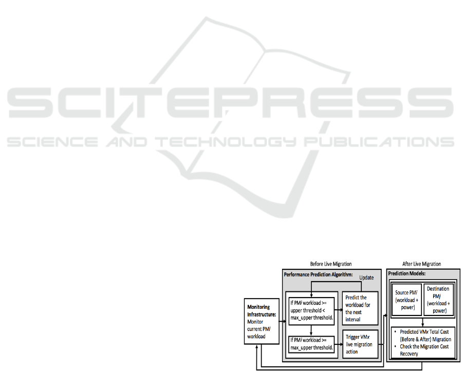
as depicted in Figure 1.
Figure 1: Performance and Energy-based Cost Prediction
Framework.
Performance and Energy-based Cost Prediction of Virtual Machines Live Migration in Clouds
385

To achieve this aim, several steps are required in
order to predict the PMs/VMs workload and power
consumption, then estimate the total cost of the
migrated VMs as explained below. The list of
parameters and their notations is shown in Table 1.
Step 1: to monitor the PMi workload, monitoring
system is used. The max_upper and upper thresholds
(e.g. 85% and 75%) are set. If the PMi workload
equals or exceeds the max_upper threshold (e.g.
85%), VM live migration is performed as shown in
Algorithm 1.
Step 2: if the PMi workload equal or exceeds the
upper threshold (e.g. 75%) but is less than the
max_upper threshold (e.g. 85%), then predict the PMi
workload for the next time interval (e.g. every 5
minutes) using the ARIMA model based on historical
workload patterns. This prediction helps detect the
workload and avoid unnecessary migration caused by
the small peaks in the workload (false alert). If the
predicted workload for the next interval exceeds the
max_upper threshold, VM live migration is
performed as shown in Algorithm 1.
Table 1: List of parameters and their notations.
PMi
PMj
VMx
C_CPU_PM
C_RAM_PM
U_CPU_PM
U_RAM_PM
C_CPU_VM
C_RAM_VM
U_CPU_VM
U_RAM_VM
the source PM
the destination PM
the candidate VM to migrate
total CPU capacity of the PM
total memory capacity of the PM
used CPU capacity of the PM (
))
used memory capacity of the PM (
))
total CPU capacity of the VM
total memory capacity of the VM
used CPU capacity of the VM
used memory capacity of the VM
Algorithm 1: Performance Prediction.
Initialise: PMi workload =
+
;
PMi max_upper threshold = 0.85 (C_CPU_ PMi, C_RAM_ PMi);
PMi upper threshold = 0.75 (C_CPU_ PMi, C_RAM_ PMi);
Predicted workload = null.
Input: PMs list.
1: for each (PMi in PMs list) do
2: if (PMi workload PMi max_upper threshold) then
3: {perform VM live migration using (Algorithm 2); break.}
4: else
5: if (PMi workload PMi upper threshold) &&
(PMi workload PMi max_upper threshold) then
6: Predicted workload predict the (PMi workload) for the
next interval using the ARIMA model.
7: PMi workload = Predicted workload;
8: end if
9: end if
10: end for
Step 3: the proposed Algorithm 2 is used to
identify the candidate VMx to be migrated and the
destination PMj to host it. The PMs are ranked in
increasing order according to their workload whereas
the VMs are ranked in decreasing order of their
workload. Starting with the PMj with the lowest
workload, the task is to select a matching candidate
VMx for migration, considering firstly the one with
the highest workload. This ensures 1) the candidate
VMx does not overload the destination PMj, and 2)
the source PMi workload decreases significantly once
migration has taken place.
Algorithm 2: VM Selection for Migration and PM
Allocation.
Initialise: VMx workload =
+
PMj workload =
+
;
PMj max_upper threshold = 0.85 (C_CPU_ PMj, C_RAM_ PMj);
PM power =
; // to check the energy efficiency.
Destination PMj = null, Candidate VMx = null.
Input: PMs list, VMs list.
Output: Candidate VMx, Destination PMj.
1: Sort the PMs list in increasing order of the workload;
2: Sort the VMs list on PMi in a decreasing order of the workload;
3: for each (PMj in PMs list) do
4: for each (VMx in VMs list) do
5: if (PM power 1) && ((PMj workload + VMx workload)
PMj max_upper threshold) then
{Destination PMj = PMj; Candidate VMx = VMx; break.}
6: end if
7: end for
8: end for
9: return (Candidate VMx, Destination PMj).
After identifying the candidate VMx and the
destination PMj, ARIMA model is used to predict the
candidate VMx workload (including CPU, memory,
disk and network) utilisation and identify the best fit
model. The ARIMA model is a time series prediction
model that has been used widely in different domains,
including finance, owing to its sophistication and
accuracy. Unlike other prediction methods, like
sample average, ARIMA takes multiple inputs as
historical observations and outputs multiple future
observations depicting the seasonal trend; further
details about the ARIMA model can be found in (Box
et al., 2015). Once the candidate VMx workload is
predicted using the ARIMA model based on historical
data, the next step is to predict the PMs workload and
PMs/VMx power consumption using regression
models. Before predicting the power consumption for
PMs/VMx, understanding how the resource usage
affects the power consumption is required. Therefore,
an experimental study is setup to investigate the
effects of the resource usage on the power
consumption. An experiment was carried out on a
local Cloud Testbed (see Section 4), and the findings
show that the CPU utilisation correlates well with the
power consumption, as supported, for example, by
(Dargie, 2015).
Step 4: to predict the PMs workload represented
as (PMs CPU utilisation), would require measuring
the relationship between the number of Virtual CPUs
CLOSER 2018 - 8th International Conference on Cloud Computing and Services Science
386
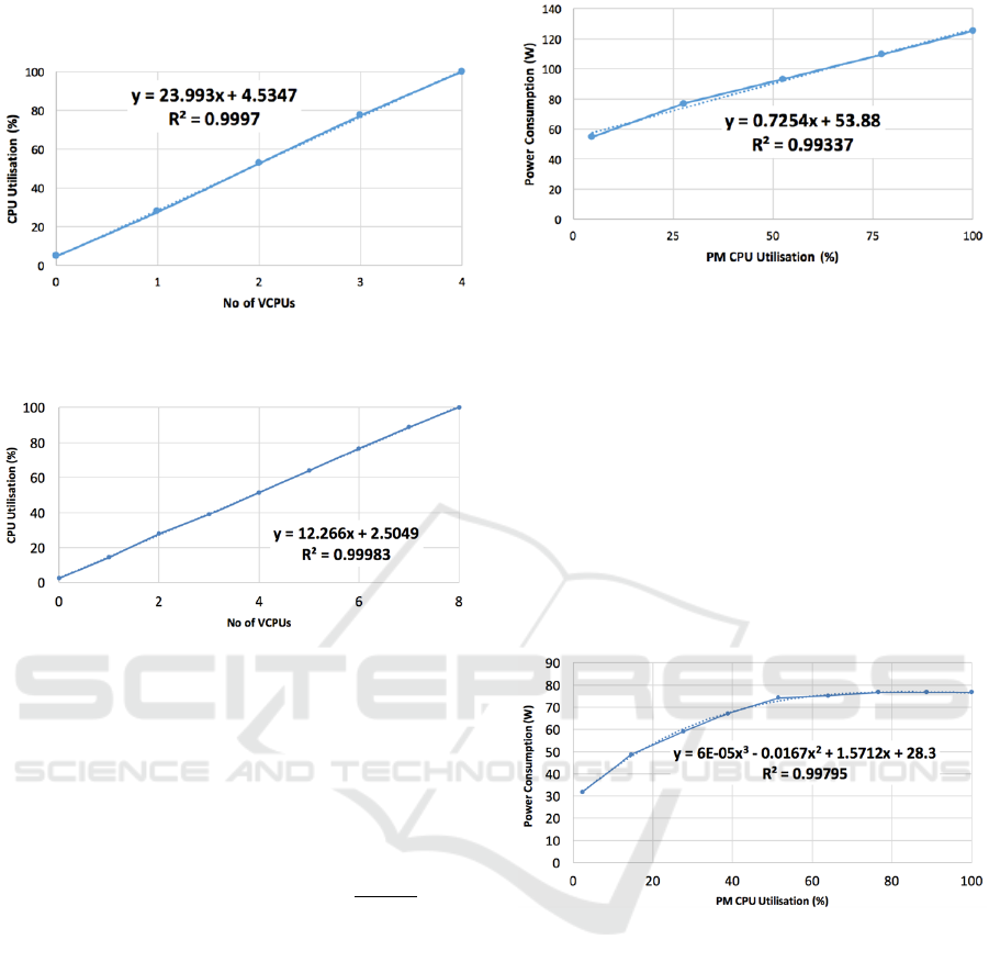
(vCPU) and the PM CPU utilisation for the PMs, as
shown in Figures 2 and 3.
Figure 2: Number of vCPUs (VMx) vs PM CPU Utilisation
(Source PMi).
Figure 3: Number of vCPUs (VMx) vs PM CPU Utilisation
(Destination PMj).
A linear regression model has been applied to
predict the PMs CPU utilisation based on the used
ratio of the requested number of vCPU for the VMx
with consideration of its current workload as the PMs
may be running other VMs already (Alzamil and
Djemame, 2016). The following equation is used (1):
(1)
is the predicted PMi CPU utilisation;
is the slope and is the intercept of the CPU
utilisation
. The
is the number of
requested vCPU for each VM and
is the
predicted utilisation for each VM. The
is
the current PMi utilisation and
is the idle
PMi utilisation. Consequently, the workload for the
destination PMj will be predicted using Equation 1,
but substituting PMi with PMj.
Step 5: the PMi power consumption is predicted
based on the relationship between the predicted PMi
workload (PMi CPU utilisation) with PMi power
consumption on the PMi. Using a regression analysis,
the relation is best described as linear regression for
this particular PMi, as shown in Figure 4.
Figure 4: The PM CPU Utilisation vs Power Consumption
(Source PMi).
Thus, the predicted PMi power consumption
measured by Watt, can be identified using
the following formula (2).
(2)
Where is the slope, is the intercept and
is predicted PMi CPU utilisation.
In the destination PMj using a regression analysis,
the relation is best described using a polynomial
model with order three for this particular PMj, as
shown in Figure 5.
Figure 5: The PM CPU Utilisation vs Power Consumption
(Destination PMj).
Thus, the predicted PMj power consumption
measured by Watt, can be identified using
the following formula (3).
Where , and are all slopes, is the intercept
and
is predicted PMj CPU utilisation.
Step 6: based on the requested number of vCPU
and the predicted vCPU utilisation, the VMx power
consumption is predicted on PMi using the proposed
formula, as shown in equation (4).
(3)
Performance and Energy-based Cost Prediction of Virtual Machines Live Migration in Clouds
387

(4)
Where
is the predicted power
consumption for VMx running on the PMi measured
by Watt.
is the requested number of
vCPU and
is the predicted VM CPU
utilisation.
is the total
requested number of vCPU for all VMs on the PMi.
is the idle power consumption and
is the predicted power consumption for
PMi. Hence, the VMx power consumption on the
destination PMj will be predicted using Equation 4,
but substituting PMi with PMj.
The energy providers usually charge by the
Kilowatt per hour (kWh). Therefore, the conversion
of the power to energy
is required
using the following equation (5):
(5)
Substituting PMi with PMj to get the energy
consumption for the VMx on the destination PMj.
Step 7: this step predicts the total cost for the
migrated VMx based on the predicted VMx resource
usage in step 3 and the predicted VMx energy
consumption in step 6.
The total time required for migrating the VMx can be
given by:
(6)
(7)
(8)
where
is the VMx total migration time measured
by seconds.
is the time when the migration
is started and
is the time when the migration
is ended.
is the running time of the VMx on
the PMi before migration starts plus the migration
time
itself and
is the running time
of the VMx before migration.
is the running
time of the VMx on the PMj during and after
migration and
is the running time of
the VMx after migration.
To predict the total cost for VMx before
migration, equation (9) is proposed:
(9)
where
is the predicted total cost
of the VMx before and during migration on the source
PMi.
is the predicted resource usage
of RAM times the cost for that resource for a period
of time. We consider the similar notation for the CPU,
disk and network resources on PMi.
is
the predicted energy consumption of the VMx times
the electricity cost as announced by the energy
providers. Thus, the total cost of the VMx during and
after migration on the destination PMj will be
predicted using Equation 9, but substituting PMi with
PMj and so on for each resource such as CPU, RAM,
disk, network and energy.
Step 8: finally, this step compares the predicted
total cost of VMx before live migration with the
predicted total cost of the same VMx after live
migration, in order to check the ability to recover the
costs incurred by live migration, as shown in
Algorithm 3.
Algorithm 3: Migration Cost Recovery.
Initialise: VMx Cost Before Migration =
;
VMx Cost After Migration =
. [as explained in Section
3. Step 7].
Input: VMs list.
Output: Boolean Cost Recovery list.
1: for each (VMx in VMs list) do
2: if (VMx Cost After Migration VMx Cost Before Migration) then
3: Cost Recovery list = true; // The cost of migration is recovered.
4: else
5: Cost Recovery list = false; // The cost of migration is not
recovered.
6: end if
7: end for
8: return Cost Recovery list.
4 EXPERIMENTAL SETUP
This section describes the environment and the details
of the experiments conducted in order to evaluate the
proposed Performance and Energy-based Cost
Prediction Framework. The prediction process starts
by firstly predicting the PMs/VMs workload using the
CLOSER 2018 - 8th International Conference on Cloud Computing and Services Science
388
(auto.arima) function in R package
2
and then
completing the cycle of the framework and
considering the correlation between the physical and
virtual resources to predict power consumption of the
VMs on a multiple PMs. After that, the total cost is
predicted for the VMs based on their predicted
workload and power consumption.
A number of experiments have been designed and
implemented on a local Cloud Testbed with the
support of the Virtual Infrastructure Manager (VIM),
OpenNebula
3
version 4.10, and KVM hypervisor for
the Virtual Machine Manager (VMM). This Cloud
Testbed includes a cluster of 8 commodity Dell
servers, and two of these servers with four core
X3430 and eight core E31230 V2 Intel Xeon CPU
were used. The servers include 16GB RAM and
1000GB hard drives. Also, each server has a Watt
meter
4
attached to directly measure the power
consumption. Heterogeneous VMs are created and
their monitoring is performed through Zabbix
5
, which
is also used for resources usage monitoring.
Rackspace
6
is used as a reference for the VMs
configurations. Three types of VMs, small, medium
and large are provided with different capacities. The
VMs are allocated with 1, 2 and 4 vCPUs, 1, 2 and 4
GB RAM, 10 GB disk and 1 GB network,
respectively. The cost of the virtual resources are set
according to ElasticHosts
7
and VMware
8
; and the cost
of Energy according to CompareMySolar
9
.
In terms of the workload patterns, Cloud
applications can experience different workload
patterns based on the customers’ usage behaviours,
and these workload patterns consume power
differently based on the resources they utilise. Several
cloud workload patterns are identified in (Fehling et
al., 2014). The periodic workload pattern is
considered as it fits nicely with the performance
variation modelling. Thus, a number of direct
experiments have been conducted to synthetically
generate periodic workload by using Stress-ng
10
in
order to stress all resources on different types of VMs.
The generated workload of each VM type has four
time intervals of 30 minutes each. The first three
intervals will be used as the historical data set for
prediction, and the last interval will be used as the
testing data set to evaluate the predicted results.
2
http://www.r-project.org/
3
https://opennebula.org/
4
https://www.powermeterstore.com
5
https://www.zabbix.com/
6
https://www.rackspace.com/cloud/servers/pricing
5 RESULTS AND DISCUSSION
This section presents the quantitative evaluation of
the Performance and Energy-based Cost Prediction
Framework. The figures below show the predicted
results for three types of VMs, small, medium and
large, running on a multiple PMs based on historical
periodic workload pattern. Because of space
limitation, only small VM results are shown.
In Algorithm 1, when PMi is overloaded and
exceeds the predefined (upper threshold), instead of
immediately migrating VMs, the prediction model is
used to minimise the number of VM migrations and
avoid unnecessary migrations caused by the small
peaks in the workload. However, when PMi is
overloaded and exceeds the predefined (max_upper
threshold), the proposed Algorithm 2 is used to
migrate the candidate VMx, in order to reduce the
overloaded PMi and allocate the VMx on appropriate
PMj which have sufficient resources and potentially
more energy efficient. It is also checked that the
destination PMj utilisation will not exceed the
max_upper threshold for reallocating of the incoming
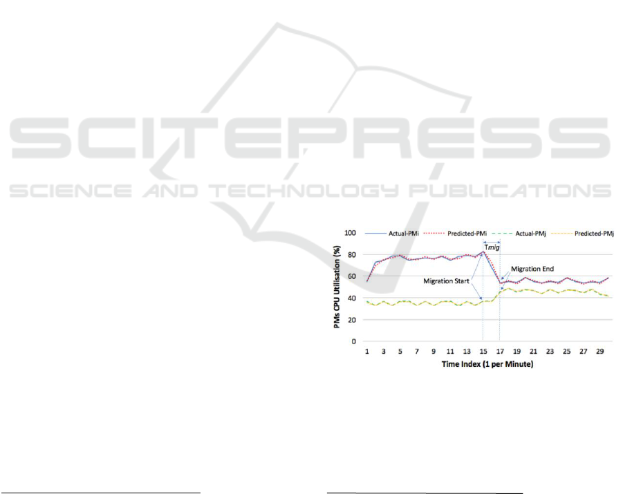
VMx. Figure 6 shows the predicted versus the actual
PMs workload when the VMs run CPU-intensive
workload. In order to achieve the live migration
without degrading the performance, both the PMi and
PMj (CPU and RAM) resources need to be carefully
managed. Since the PMi max_upper threshold (85%)
predefined and PMj have available resources to
accept the candidate VMx, thus the performance
during live migration is not affected.
Figure 6: Predicted vs Actual in both PMs (Source PMi and
Destination PMj).
Figure 7 (a, b, c and d) depict the results of the
migrated VMx predicted versus the actual workload,
including CPU, RAM, disk, and network usage for
7
https://www.elastichosts.co.uk/pricing/
8
https://www.vmware.com/cloud-services/pricing-guide
9
http://blog.comparemysolar.co.uk/electricity-price-per-
kwh-comparison-of-big-six-energy-companies/
10
http://kernel.ubuntu.com/~cking/stress-ng/
Performance and Energy-based Cost Prediction of Virtual Machines Live Migration in Clouds
389
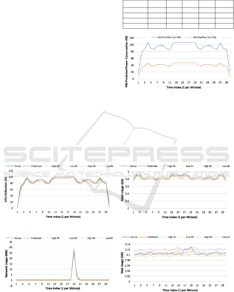
the VMx. Despite the periodic utilisation peaks, the
predicted VMx CPU, RAM and network workload
results closely match the actual results, which reflects
the capability of the ARIMA model to capture the
historical seasonal trend and give a very accurate
prediction accordingly. The predicted VMx disk
workload is also matching the actual workload, but
with less accuracy as compared to the CPU, RAM and
network prediction results. This can be justified
because of the high variations in the generated
historical periodic workload pattern of the disk not
closely matching in each interval. Beside the
predicted mean values, the figures also show the high
and low 95% and 80% confidence intervals.
In terms of prediction accuracy, a number of
metrics have been used to evaluate the results, such
as Mean Error (ME), Root Mean Squared Error
(RMSE), Mean Absolute Error (MAE), Mean
Percentage Error (MPE), and Mean Absolute
Percent Error (MAPE); further details about these
accuracy metrics can be found in (Hyndman and
Athanasopoulos, 2013). The accuracy of the
predicted VMs workload (CPU, RAM, disk, network)
based on periodic workload is evaluated using these
accuracy metrics, as summarised in Table 2.
Table 2: Prediction Accuracy for a Small VM.
Parameters
ME
RMSE
MAE
MPE
MAPE
CPU
0.00486
1.7101
0.5652
-3.4611
4.978
RAM
0.00167
0.0189
0.0055
0.1618
0.6585
Disk
0.00072
0.0051
0.0030
0.64200
2.8612
Network
-0.0052
0.1869
0.0461
31.459
60.940
Figure 7: Predicted VMx Power Consumption on (Source
PMi and Destination PMj).
The proposed framework can predict the power
consumption for a number of VMs when running on
source PMi and destination PMj (based on Step 6,
Equation 4 in Section 3), noting that the PMj is more
energy efficient than PMi as shown in Figure 8. The
predicted power consumption attribution for each
VM is affected by the variation in the predicted CPU
utilisation of all the VMs.
(a)
(b)
(c)
(d)
Figure 8: The Prediction Results for a Small VMx.
CLOSER 2018 - 8th International Conference on Cloud Computing and Services Science
390
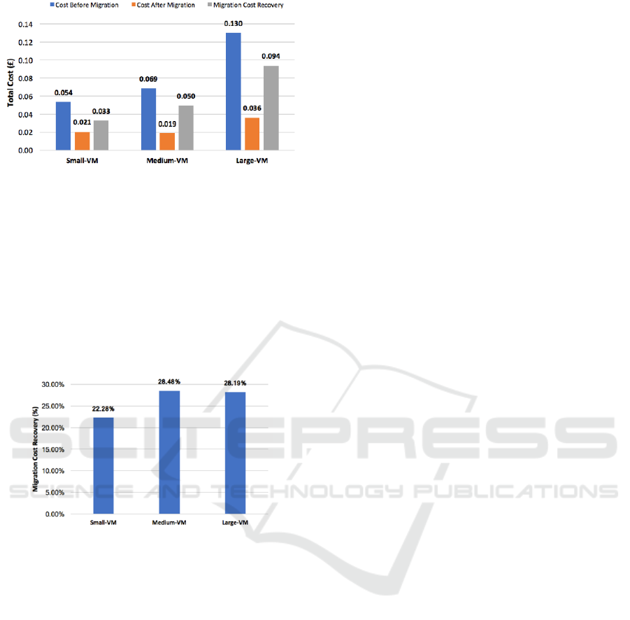
Figure 9: Predicted Total Cost Before vs After Migration
with The Migration Cost Recovery.
This framework is also capable of predicting the
total cost before and after live migration for a number
of VMs as shown in Figure 9, along with their
migration cost recovery based on Algorithm 3.
In addition, Figure 10 shows the results of the
predicted migration cost recovery for all VMs with
(the cost recovery percentage incurred by live
migration): 22.28% for the small VM, 28.48% for the
medium and 28.19% for the large one.
Figure 10: The Potential Migration Cost Recovery.
Despite the high variation of the workload
utilisation in the periodic pattern, the accuracy metrics
indicate that the predicted VMs workload and power
consumption achieve good prediction accuracy along
with the predicted live migration total cost.
6 CONCLUSION AND FUTURE
WORK
This paper has presented and evaluated a new
Performance and Energy-based Cost Prediction
Framework that dynamically supports VMs
reallocation, and demonstrates the trade-off between
cost, power consumption, and performance. This
framework predicts the total cost before and after live
migration by considering the resource usage, power
consumption and performance variation of
heterogeneous VMs based on their usage and size,
which reflect the physical resource usage and power
consumption by each VM. The results show that the
proposed framework can predict the resource usage,
power consumption, total migration cost and the
migration recovery cost for the VMs with a good
prediction accuracy based on periodic workload
patterns. As a part of future work, we intend to extend
our approach by considering the scalability aspects
(auto-scaling) to further understand the capability of
the proposed work.
REFERENCES
Aldossary, M., Alzamil, I. and Djemame, K. (2017)
‘Towards Virtual Machine Energy-Aware Cost
Prediction in Clouds’, in GECON 2017, pp. 119–131.
Alzamil, I. and Djemame, K. (2016) ‘Energy Prediction for
Cloud Workload Patterns’, in GECON 2016, pp.160–
174.
Box, G. E. P., Jenkins, G. M., Reinsel, G. C. and Ljung, G.
M. (2015) Time series analysis: forecasting and
control. John Wiley & Sons.
Dargie, W. (2015) ‘A stochastic model for estimating the
power consumption of a processor’, Computers, IEEE
Transactions on, pp. 1311–1322.
Fehling, C., Leymann, F., Retter, R., Schupeck, W. and
Arbitter, P. (2014) Cloud Computing Patterns.
Hyndman, R. J. and Athanasopoulos, G. (2013) Measuring
forecast accuracy, OTexts. Available at: at
www.otexts.org/fpp/2/5 (Accessed: 1 October 2017).
Liu, H., Jin, H., Xu, C.-Z. and Liao, X. (2013) ‘Performance
and energy modeling for live migration of virtual
machines’, Cluster Computing, 16(2), pp. 249–264.
Melhem, S. B., Agarwal, A., Goel, N. and Zaman, M.
(2017) ‘Selection process approaches in live migration:
A comparative study’, in ICICS 2017, pp. 23–28.
Raghunath, B. R. and Annappa B. (2017) ‘Prediction based
dynamic resource provisioning in virtualized
environments’, in ICCE 2017, pp. 100–105.
Strunk, A. (2012) ‘Costs of virtual machine live migration:
A survey’, in Proceedings - 2012 IEEE 8th World
Congress on Services, pp. 323–329.
Strunk, A. (2013) ‘A lightweight model for estimating
energy cost of live migration of virtual machines’, in
IEEE International Conference on Cloud Computing,
CLOUD, pp. 510–517.
Voorsluys, W., Broberg, J., Venugopal, S. and Buyya, R.
(2009) ‘Cost of virtual machine live migration in
clouds: A performance evaluation’, in Lecture Notes in
Computer Science (including subseries Lecture Notes
in Artificial Intelligence and Lecture Notes in
Bioinformatics), pp. 254–265.
Xu, F., Liu, F. and Jin, H. (2016) ‘Heterogeneity and
Interference-Aware Virtual Machine Provisioning for
Predictable Performance in the Cloud’, IEEE
Transactions on Computers, 65(8), pp. 2470–2483.
Performance and Energy-based Cost Prediction of Virtual Machines Live Migration in Clouds
391
