Forecasting Short-term Solar Radiation for

Photovoltaic Energy Predictions

Alessandro Aliberti

, Lorenzo Bottaccioli

, Giansalvo Cirrincione

Enrico Macii

, Andrea Acquaviva

and Edoardo Patti

Dept. of Control and Computer Engineering, Politecnico di Torino, Torino, Italy

Universite de Picardie Jules Verne, Amiens, France

{giansalvo.cirrincione}@u-picardie.fr

Keywords:

Solar Radiation Forecast, Artiﬁcial Neural Networks, Photovoltaic System, Energy Forecast, Renewable

Energy.

Abstract:

In the world, energy demand continues to grow incessantly. At the same time, there is a growing need to

reduce CO

emissions, greenhouse effects and pollution in our cities. A viable solution consists in producing

energy by exploiting renewable sources, such as solar energy. However, for the efﬁcient use of this energy,

accurate estimation methods are needed. Indeed, applications like Demand/Response require prediction tools

to estimate the generation proﬁles of renewable energy sources.

This paper presents an innovative methodology for short-term (e.g. 15 minutes) forecasting of Global Ho-

rizontal Solar Irradiance (GHI). The proposed methodology is based on a Non-linear Autoregressive neural

network. This neural network has been trained and validated with a dataset consisting of solar radiation sam-

ples collected for four years by a real weather station. Then GHI forecast, the output of the neural network, is

given as input to our Photovoltaic simulator to predict energy production in short-term time periods. Finally,

experimental results for both GHI forecast and Photovoltaic energy prediction are presented and discussed.

1 INTRODUCTION

The widespread development of Renewable Energy

Sources (RES) in our cities, such as Photovoltaic (PV)

systems, is changing the electrical energy production,

consumption and distribution. Our society is facing

the transition from centralized and hierarchical po-

wer distribution systems to distributed and coopera-

tive ones, generally called Smart Grids. Smart Grid

technologies are opening the electrical marketplace

to new actors (e.g. prosumers and energy aggrega-

tors). Currently, power grid stability is achieved by

classic generation plants using primary and secon-

dary reserve at large-scale. Whilst, in a Smart Grid

scenario, such a new actors can actively contribute to

load balancing by fostering novel services for network

management and stability. Demand/Response (Siano,

2014) is an example of application for Smart Grid

management. It permits achieving a temporary vir-

tual power plant (Vardakas et al., 2015) by changing

the energy consumption pattern of consumers to ma-

tch RES energy production or to fulﬁl grid operation

requirements. This process is generally done every

15 minutes. To achieve these goals, prediction tools

for both RES energy generation and consumption are

needed.

In this work, we present a methodology for Pho-

tovoltaic energy prediction starting from forecasting

short-term solar radiation. The forecast of solar radi-

ation is obtained exploiting a Nonlinear Autoregres-

sive neural network. We trained and validated this

neural network with a dataset consisting of four ye-

ars of Global Horizontal Solar Irradiance (GHI) sam-

ples collected by a real weather station. The neural

network is a Multilayer Perceptron exploiting a high

number of regressors to predict GHI in 15 minutes up

to 2 hours range. Then, GHI forecast is given as input

to our PV simulator that exploits GIS tools for simu-

lating energy production. The rest of the paper is or-

ganized as follows. Section 2 reviews literature solu-

tion on solar radiation forecast. Section 3 introduces

the followed methodology to deﬁne a neural network

for short-term solar radiation forecasting. Section 4

details all the steps performed to initialize, train and

validate our neural network. Section 5 discusses the

results on solar radiation forecast. Section 6 descri-

Aliberti, A., Bottaccioli, L., Cirrincione, G., Macii, E., Acquaviva, A. and Patti, E.

Forecasting Short-term Solar Radiation for Photovoltaic Energy Predictions.

DOI: 10.5220/0006683600440053

In Proceedings of the 7th International Conference on Smart Cities and Green ICT Systems (SMARTGREENS 2018), pages 44-53

ISBN: 978-989-758-292-9

bes the adopted Photovoltaic simulator. Section 6 pre-

sents also results and accuracy on PV energy genera-

tion that exploits foretasted solar radiation given by

the proposed neural network. Finally, Section 7 dis-

cusses concluding remarks.

2 RELATED WORK

Nowadays, solar energy represents a very attractive

solution to produce green and clean energy. However,

for an efﬁcient conversion and utilization of solar po-

wer, solar radiation should be estimated and forecas-

ted through accurate methods and tools. For exam-

ple in Demand/Response applications (Siano, 2014),

the amount of available energy must be known in ad-

vance to optimize the production of power plants (Ag-

haei and Alizadeh, 2013) and to match energy pro-

duction with consumption. Hence, several studies

were proposed in the literature to ﬁnd mathematical

and physical models to estimate and forecast the so-

lar radiation, such as stochastic models based on time

series (Kaplanis and Kaplani, 2016), (Voyant et al.,

2014) and (Badescu, 2014). Moreover, classical li-

near time series models, like autoregressive moving

average, have been widely used (Brockwell and Da-

vis, 2016). However, it has been proven that these

methodologies often are not sufﬁcient in the analy-

sis and prediction of solar radiation. This is due to

the non-stationary and non-linearity of the solar radi-

ation time series data (Madanchi et al., 2017), (Naza-

ripouya et al., 2016). Furthermore, stochastic models

are based on the probability estimation. This leads to

a difﬁcult forecast of the solar radiation time series.

To overcome these limits, non-linear approaches,

such as artiﬁcial neural networks (ANNs), were con-

sidered by many researchers as powerful methodo-

logies to predict phenomenons, such as solar radia-

tion (Voyant et al., 2017). Generally, ANNs do not re-

quire knowledge of internal system parameters. Furt-

hermore, these models offer a compact solution for

multiple variable problem (Qazi et al., 2015). Howe-

ver, also the use of an ANN to forecast a phenomenon

introduces an error, the so-called prediction error (Ya-

dav and Chandel, 2014). As a result, these models

need optimizations to reduce this error.

With respect to literature solutions, the scienti-

ﬁc novelty of the proposed methodology consists in

using a neural network based on the Multilayer Per-

ceptron to forecast solar radiation. Generally, most

literature methodologies rely on the single past value

to perform the forecast (Box et al., 2015). Whilst, the

proposed solution allows to reduce signiﬁcantly the

prediction error by using a high number of regressors

to perform predictions. In addition, we perform the

forecast of solar radiation in short- and medium-term,

i.e. from future 15 minutes up to next 2 hours.

3 METHODOLOGY

A time series identiﬁes an ordered sequence of values

of a variable at equally spaced time intervals (Hamil-

ton, 1994). The usage of time series models brings

two great beneﬁts: i) understanding the underlying

forces and structure that produced the observed data

and ii) ﬁtting a model and proceeding to forecast

and monitor or even feedback and feed-forward cont-

rol (Oancea and Ciucu, 2014).

3.1 The Multilayer Perceptron

Generally, one of the most effective methods for pre-

diction based on time series consists in neural net-

work (Montgomery et al., 2015), such as the Multi-

layer Perceptron (MLP), which is the artiﬁcial neu-

ral network most used in applications (Demuth et al.,

2014). It is composed of units, called nodes or neu-

rons, and organized in a layer of inputs, one or more

hidden layers and an output layer. It is a feed-forward

network with full connection between layers. The

connections are characterized by adjustable parame-

ters called weights. Hence, a weight refers to the

strength of a connection between two nodes (Kubat,

2017). Each neuron computes a function of the sum

of the weighted inputs. This function is called activa-

tion function.

In this work, we use an MLP-network architec-

ture characterized by i) one hidden layer of neurons

with hyperbolic tangent activation function f and ii)

an output layer with a linear activation function F.

The functional model is given by:

ˆy

(w,W) = F

(

∑

j=1

i j

) =

= F

(

∑

j=0

i j

(

∑

l=1

+ w

) +W

)

(1)

The weights are speciﬁed by the matrix W = [W

i j

] and

by the matrix w = [w

], where W

i j

scales the con-

nection between the hidden unit j and the output unit

i and w

scales the connection between the hidden

unit j and the input unit l. W

and w

are the cor-

responding biases. All this weights can be vectorized

in a vector θ. The input units are represented by the

vector u(t) and the hidden neuron outputs are repre-

sented by the vector h. The outputs of the network,

Forecasting Short-term Solar Radiation for Photovoltaic Energy Predictions

ˆy

, are estimated by Eq. 1. The parameters are deter-

mined during the training process, which requires a

training set Z

, composed of a set of inputs, u(t), and

corresponding desired outputs, y(t), speciﬁed by:

= [u(t), y(t)], t = 1, ..., N (2)

The training phase allows to determine a mapping

from the set of training data to the set of possible

weights:

→

θ (3)

so that the network can produce prediction ˆy(t), to be

compared to the true output y(t).

The prediction error approach is instead based on

the introduction of a measure of closeness in terms of

a mean square error criterion, as speciﬁed by:

(θ, Z

) =

∑

t=1

[y(t)− ˆy(t|θ)]

[y(t)− ˆy(t|θ)] (4)

The weights are then found as:

θ = arg

minV

(θ, Z

) (5)

by some kind of iterative minimization scheme:

i+1

= θ

+ µ

+ f

(6)

where θ

speciﬁes the current iteration, f

the search

direction and µ

the step size.

3.2 System Identiﬁcation

The following section details the adopted methodo-

logy to use an artiﬁcial neural network for short-term

solar radiation predictions. Based on the process pre-

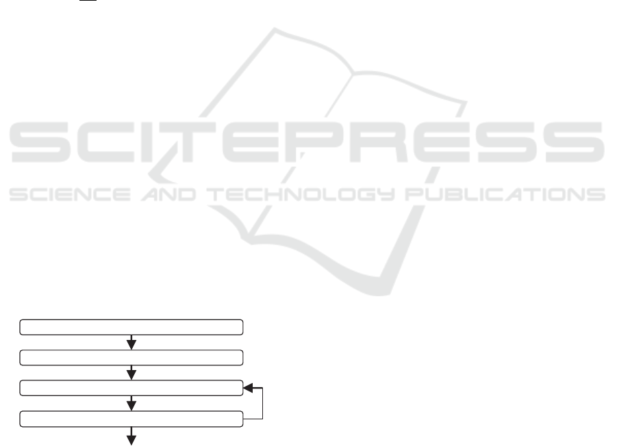
sented in (Norgaard et al., 2000), the procedure to

identify a dynamical system consists of four steps: i)

Experiment, ii) Model Structure Selection, iii) Model

Estimation and iv) Model Validation (see Fig. 1).

OPTIMIZATION

EXPERIMENT

SELECT MODEL STRUCTURE

ESTIMATE MODEL

VALIDATE MODEL

VALIDATION

Figure 1: System identiﬁcation procedure.

Experiment. This step corresponds to the problem

analysis and the sampling and data collection. In

neural network applications, once the scope has been

identiﬁed, an adequate amount of data is needed. Ge-

nerally, an higher number of data allows better fore-

casting performances (Srivastava et al., 2014). Then

the available data must be divided into two different

datasets: the training set and the validation set, re-

spectively. These datasets are used in the training and

validation phases of the neural network, which are

the Estimate Model and the Validate Model steps in

Fig. 1, respectively.

Model Structure Selection. This step allows iden-

tifying the correct architecture model to use (Nor-

gaard et al., 2000). Generally, this selection is

more difﬁcult in the nonlinear case than in the li-

near (Chandrashekar and Sahin, 2014). At this aim,

the system regressor must be studied. In mathema-

tical modeling, these regressors identify independent

variables able to inﬂuence the dependent variables. In

time series, then, these regressors represent previous

samplings with respect to the predicted ones (Mont-

gomery et al., 2015). Consequently, the best neural

structure can be chosen.

Model Estimation. In this step, once the network

model and the number of regressors are identiﬁed, the

network is ﬁrst implemented and then trained. In time

series scenario, training a neural network is needed to

provide: i) the vector containing desired output data;

ii) the number of regressors to deﬁne the prediction;

iii) the vector containing the weights of both input-

to-hidden and hidden-to-output layers and lastly iv)

the data structure containing the parameters associa-

ted with the selected training algorithm. Finally, the

training phase produces a training error, which re-

presents the network performance index (Srivastava

et al., 2014).

Model Validation. This step validates the trained

network. Generally, validating a network allows eva-

luating its capabilities (Miller et al., 1989). In time

series predictions, the most common validation met-

hod consists of analysing the residuals (i.e. prediction

errors) by cross-validating the test set. This method

allows to perform a set of tests including also the au-

tocorrelation function of the residuals and the cross-

correlation function between controls and residuals.

This analysis provides the test error (Srivastava et al.,

2014), that is an index considered as a generalization

of the error estimation. This index should not be too

high compared to training error. If this happens, the

network could over-ﬁt the training set.

Network Optimization and Final Validation. Ge-

nerally, if the network is over-ﬁtting the training set,

the selected model structure contains too many weig-

hts. It is required to return in the Estimate Model step

in order to change and redeﬁne some structural para-

meters by optimizing the whole architecture. For this

purpose, the superﬂuous weight must be pruned ac-

cording to the Optimal Brain Surgeon (OBS) strategy,

SMARTGREENS 2018 - 7th International Conference on Smart Cities and Green ICT Systems

that represents one of the most important optimization

strategies (Han et al., 2015). Consequently, once the

new weights are given, the network architecture must

be re-validated.

4 NAR NEURAL NETWORK FOR

SHORT-TERM GHI FORECAST

In this work, we aim at forecasting the short-term

Global Horizontal Solar Irradiance (GHI) for photo-

voltaic energy predictions. For this purpose, we used

a dataset of about four years (from 2010 to 2013).

It provides GHI values sampled every 15 minutes by

the weather station in our University Campus. In de-

tail, we considered all values in the time period from

8 a.m. to 6 p.m. Thus, we excluded evening and

night time. Then, we split the dataset into training

set (2010-2011) and validation set (2012-2013). This

dataset appears to be statistically relevant. Nonet-

heless, we believe that if we could have used a lar-

ger accurate training set we could have achieved even

more accurate prediction results. In order to deal with

time series data, we adopted the Nonlinear Autore-

gressive neural network (NAR) belonging to the Non-

linear Autoregressive Exogenous Model (NARX) fa-

mily (Siegelmann et al., 1997). Other choices, like

NARMA (Norgaard et al., 2000) are possible. Howe-

ver, NARX is considered as the best tool in time series

analysis (used as NAR) and does not suffer from sta-

bility problems. It is a nonlinear autoregressive model

which has exogenous inputs. It is basically a choice

of the inputs of a nonlinear model (an MLP neural

network, as in (Norgaard et al., 2000)), which repla-

ces the traditional linear model ARX (as in (Ljung,

1998)). It bases its predictions on i) past values of the

series and ii) current and past values of the driving

exogenous series, producing an error that represents

the error of prediction. This error means that the kno-

wledge of the past terms does not enable the future

value of the time series to be predicted exactly. These

network models are characterized by:

= F(y

t−1

, y

t−2

, y

t−3

, ..., u

, u

t−1

, u

t−2

, u

t−3

, ...) + ε

(7)

where y

represents the variable of interest and u

the externally determined variable at time t respecti-

vely. In detail, information about u

and previous va-

lues of u and y, helps predicting y

, with a prediction

error ε

Once the model has been chosen, we analysed the

number of past signals used as regressors for the pre-

diction. We used Lipschiz method for determining the

lag-space (Rajamani, 1998). This methodology al-

lows identifying the orders of Input-Output Models

for Nonlinear Dynamic Systems. However, as de-

tailed in (He and Asada, 1993), this methodology is

not always effective but it represents a good starting

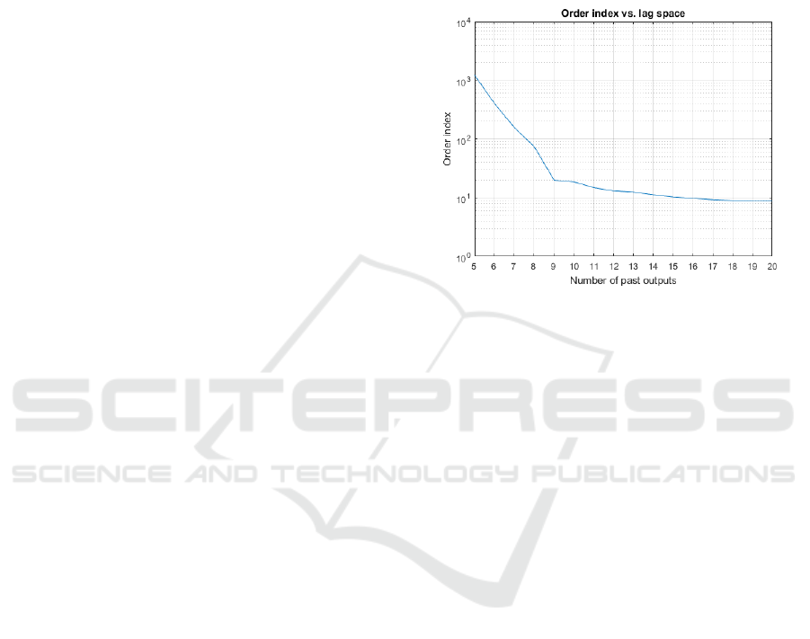
point to deﬁne the number of regressors. Fig. 2 details

the result of the applied Lipschiz method, in which

the number of past inputs is increased simultaneously

from 1 to 20.

Figure 2: Evaluation of Order Index criterion for different

lag-space.

In this way, we deduced that the architecture can yield

a good performance with only 9 regressors (i.e. 9 pre-

vious values for y and u, respectively, in Eq. 7). Ho-

wever, considering that the value of 10 is very close to

the knee of the curve, 10 regressors have been chosen

in order to have more conservative results, in the sense

of the use of more information from the time series.

Then, we chose an initial fully connected network ar-

chitecture with one hidden layer of 30 hyperbolic tan-

gent units. This large number of units is redundant,

but justiﬁed by the pruning technique. The weights

of the network are then initialized randomly before a

training. This choice allows to initialize i) the weig-

hts, ii) their decay threshold and iii) the maximum

number of iterations. However, these data structure

parameters are overestimated during the ﬁrst training.

After this phase, we proceed training the neural net-

work. Training is a minimization technique in order

to compute the best weights for the network. Here we

used the Levenberg-Marquardt algorithm, which in-

terpolates between the Gauss-Newton algorithm and

the method of gradient descent, using a trust region

approach (Norgaard et al., 2000).

According to the purpose of this study, we chose

to use the methodology illustrated in (Norgaard et al.,

2002) for the network validation. This methodo-

logy allows the models systems validation of the out-

puts, performing a set of tests including autocorre-

lation function of the residuals and cross-correlation

function between controls and residuals. This pro-

Forecasting Short-term Solar Radiation for Photovoltaic Energy Predictions

cess produces the test error index as a result. The

test error represents an estimation of the generaliza-

tion error. This should not be too large compared to

training error. If the test error (NSSE) is greater than

the training error, it means that the predicted results

are over-ﬁtting the training set. In our case, the va-

lidation process yield this index equal to 3.27 × 10

which is a good value. Then, we proceeded to the op-

timization phase of the network. Our purpose was to

remove excess weights and obtain a smaller training

error than the one given during the ﬁrst validation. In

order to do so, we adopted the Optimal Brain Surgeon

(OBS) strategy (Hansen et al., 1994), which prunes

superﬂuous weights. OBS computes the Hessian ma-

trix weights iteratively, which leads to a more exact

approximation of the error function. The inverse Hes-

sian is calculated by means of recursion. This method

allows ﬁnding the smallest saliency S

2[H

−1]

]

i,i

(8)

where [H

−1

]

i,i

is the (i, i)th element of the inverse

Hessian matrix and w

is the ith element of the vector

θ containing network weights. The saliency identi-

ﬁes the quality of the connection between the various

network units. This methodology allows to verify the

state of the saliency iteratively. If the saliency S

much smaller than the mean-square error, then some

synaptic weights are deleted and the remaining ones

are updated. The computation stops when no more

weights can be removed from the network without a

large increase of the mean-square error. Once the new

weights are given, we re-validated the network archi-

tecture.

Through the same methodology used in the ﬁrst

validation phase, we proceeded to the ﬁnal network

validation using the new weights. The resulting test

error index NSSE was 3.11 × 10

, that is lower than

the previous one. Thus, the prediction error has been

further lowered, giving more precise GHI forecast.

Fig. 3 shows the ﬁnal structure of the neural network

after the optimization process.

Figure 3: NAR optimized structure.

5 RESULTS ON GHI FORECAST

The phases of the neural network characterization

described in Section 4 allow deﬁning an architecture

that bases its prediction on 10 previous regressors.

This represents a big advantage, as in literature these

kinds of networks generally use just the single pre-

vious value to predict the next one. This implies a

higher prediction error. In our case, by using a more

large number of previous instances the prediction is

good.

Our goal is to predict GHI in very short time win-

dows (i.e. 15 minutes). We moved further predicting

also GHI up to next two hours with 15 min. time inter-

val. Using the dataset described in Section 4, we per-

form predictions by employing the methodology pre-

sented in (Norgaard et al., 2002). This methodology

allows to determine the prediction value (that corre-

sponds to the ahead k-step prediction of the system)

and compare it to the measured output. The predicti-

ons are determined i) by feeding past predictions in

the neural network where observations are not avai-

lable and ii) by setting unavailable residuals to zero.

Before starting the simulations, we set the prediction

function to 10 regressors. In this section, we present

the obtained results.

To evaluate the performance of our predicti-

ons, we used the indicators reported by Gueymard

in (Gueymard, 2014). These indices of dispersion are:

i) the Root Mean Square Difference (RMSD) that re-

presents the standard deviation of differences between

predicted and observed values; ii) the Mean Absolute

Difference (MAD) that represents a measure of sta-

tistical dispersion obtained by the average absolute

difference of two independent values drawn from a

probability distribution; iii) the Mean Bias Difference

(MBD) that measures the average squares of errors be-

tween predicted and measured values; iv) the Coefﬁ-

cient of determination (r

) that represent the propor-

tion between the variance and the predicted variable.

RMSD, MAD and MBD are expressed in percentage

rather than absolute units. Furthermore, we also con-

sidered two indicators for the overall network perfor-

mance: i) the Willmotts Index of Agreement (WIA) that

represent the standardized measure of the degree of

model prediction error (Willmott et al., 2012) and ii)

the Legatess Coefﬁcient of Efﬁciency (LCE) that is the

ratio between the mean square error and the variance

in the observed data (Legates and McCabe, 2013).

Fig. 4 shows the comparison among GHI results

given by our neural network (dashed lines) and me-

asured values sampled by the weather station (con-

tinues line) for different steps, from k = 1 (i.e next

15 min.) to k = 8 (i.e next 120 min.). These GHI

SMARTGREENS 2018 - 7th International Conference on Smart Cities and Green ICT Systems

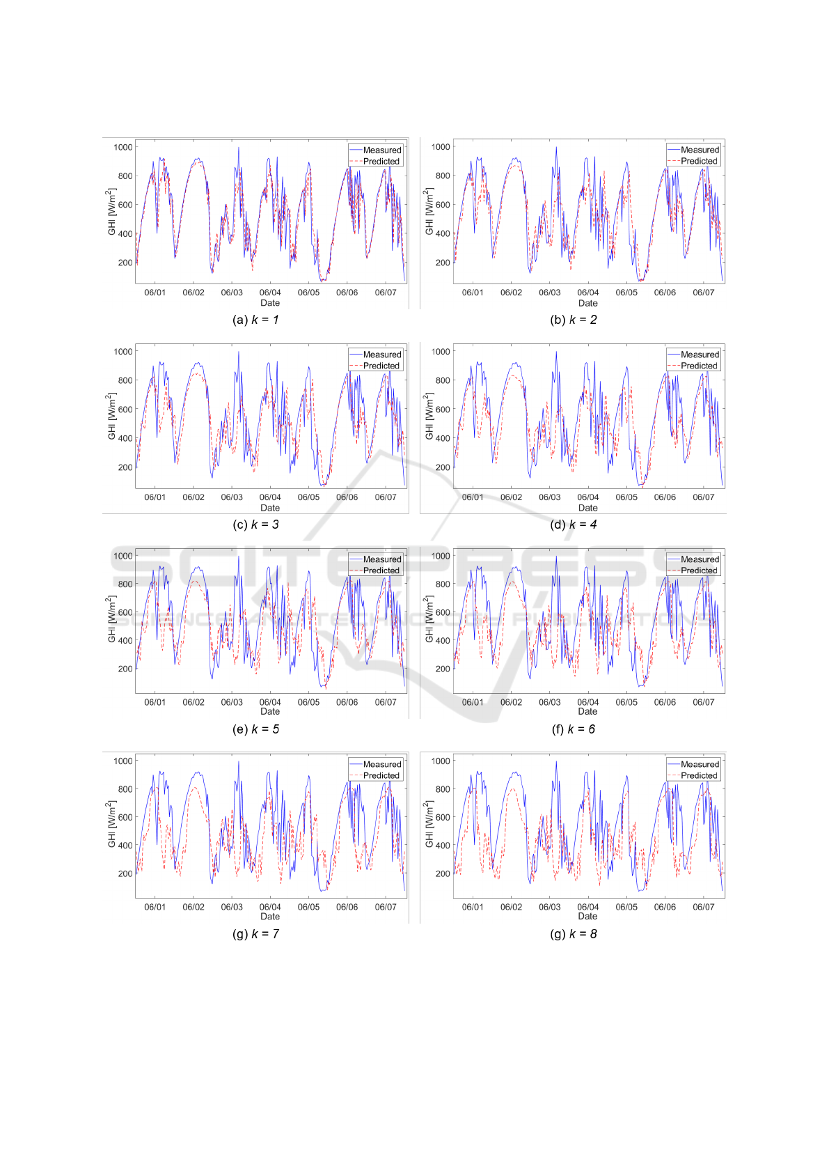
Figure 4: GHI prediction for 1 ≤ k ≤ 8 (June 2013).

Forecasting Short-term Solar Radiation for Photovoltaic Energy Predictions

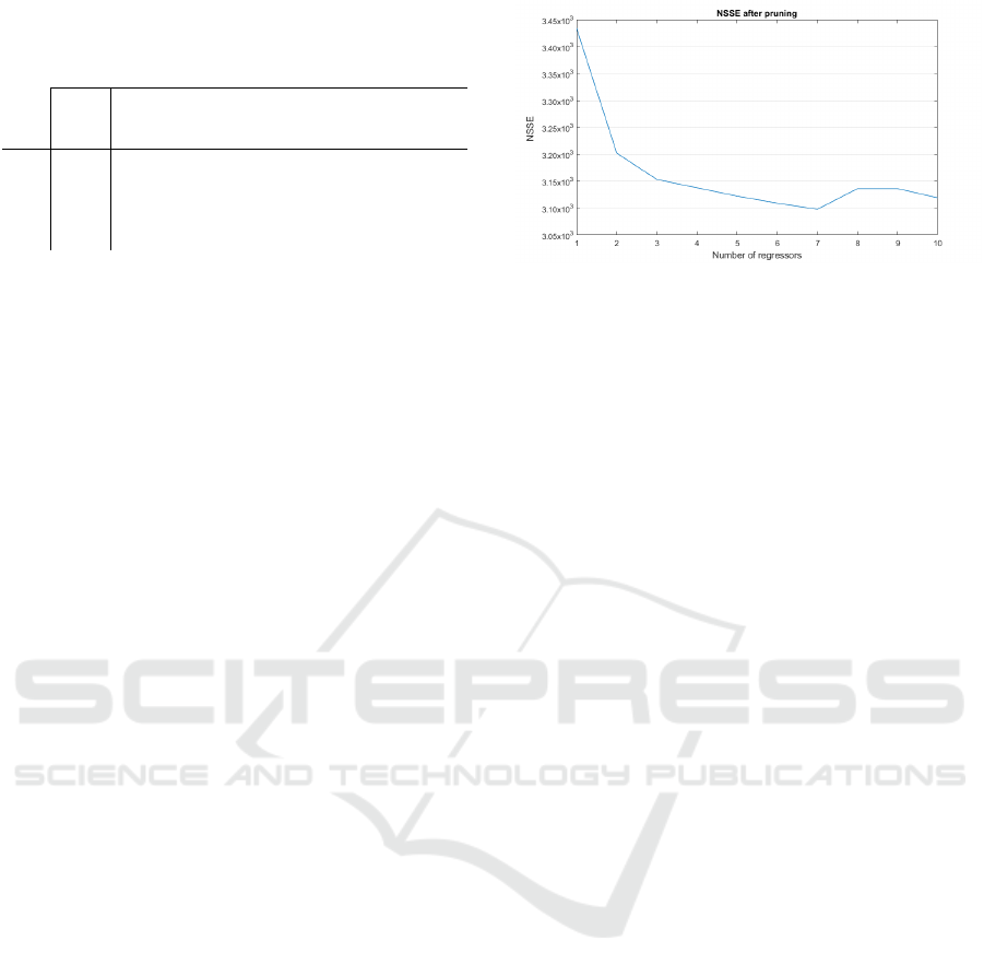
Table 1: Performance Indicators for GHI prediction.

Time

[min]

MAD

[%]

MDB

[%]

RMSD

[%]

LCE WIA

k=1 15 13.56 0.26 0.91 25.37 0.81 0.98

k=2 30 19.82 0.70 0.84 32.92 0.72 0.96

k=3 45 24.28 1.08 0.80 37.61 0.66 0.94

k=4 60 28.02 1.27 0.75 41.55 0.60 0.93

k=5 75 31.30 1.52 0.71 45.10 0.56 0.91

k=6 105 34.43 1.42 0.66 48.48 0.51 0.90

k=7 115 37.88 0.97 0.61 52.15 0.46 0.88

k=8 120 41.32 0.14 0.55 55.97 0.41 0.86

predictions refer to the ﬁrst week of June 2013. As

shown in Fig. 4-(a), Fig. 4-(b) and Fig. 4-(c), the

trends of our results for 1 ≤ k ≤ 3 follow the real GHI

behaviour with a good accuracy. Instead for k > 3,

the prediction accuracy decreases (from Fig. 4-(d) to

Fig. 4-(g)). This is also highlighted by Table 1 that

reports the results of GHI predictions in terms of per-

formance indicators considering the whole validation

set (i.e. 2012-2013).

Performance indices clearly show that the architec-

ture performance worsens by increasing the predictive

steps. As a result, GHI prediction for high values of k

has a greater error than real data. The analysis of indi-

ces highlights that the best GHI predictions are given

at smaller intervals. For example, the MAD indicates

that GHI prediction error grows as the prediction step

k increases. Indeed, for prediction step k = 1 the er-

ror is about 13.6% while for k = 8 the error is around

41%. Also, RMSD has a similar trend. Furthermore,

the coefﬁcient of determination r

is much better than

it is closer to 1. This index for prediction step k = 1

is equal to 0.91. Whilst, the error increases with an

= 0.55 for k = 8.

This is also conﬁrmed by LCE and WIA that high-

light a decreasing of the overall performance on high

prediction steps. Increasing the forecasting steps in-

crease the errors and, consequently, the performances

of prediction gets worst. Also for LCE and WIA, va-

lues closer to 1 represent the best case. For k = 8,

LCE and WIA are equal to 0.41 and 0.86, respectively.

However, the performance indexes for 1 ≤ k ≤ 3 are

acceptable to perform Photovoltaic energy estimati-

ons (see Section 6). In this scenario, the maximum

error for GHI prediction is less than 25% for k = 3.

The correctness of the choice of the number of re-

gressors by the Lipschitz method seen previously is

conﬁrmed by the following additional analysis whose

results are shown in Fig. 5. The technique proposed

here has been repeated for different numbers of in-

puts and the corresponding NSSE has been recorded.

It can be seen that too few regressors are not enough

and seven or ten inputs give the best results. It con-

ﬁrms the choice in the proposed experiment.

Figure 5: Evaluation of NSSE after pruning with regard to

the number of regressors.

6 PV ENERGY ESTIMATION

As discussed in Section 5, the results on GHI fore-

cast are satisfactory especially on short-term time pe-

riods. This forecast of GHI allows estimating in ad-

vance the energy production of renewable, such as PV

systems. In our case, we used GHI predictions as

input to our PV energy simulator (Bottaccioli et al.,

2017b). Estimating the PV production for the next

short-term time windows enables the development of

more accurate control policies for Smart Grid ma-

nagement, such as Demand/Response (Siano, 2014).

Furthermore, this estimation allows to analyse the pe-

netration level and the impact of renewable energy in

existing districts and smart grids and. Also, to test and

validate complex systems as presented in (Bottaccioli

et al., 2017a).

6.1 PV Simulator

This work exploits the software infrastructure presen-

ted in our previous work (Bottaccioli et al., 2017b) to

estimate the energy generation proﬁles of PV systems

in real-sky conditions. The inputs of this simulator are

i) a Digital Surface Model (DSM) and ii) GHI trends.

The DSM is a high-resolution raster image represen-

ting terrain elevation of buildings of interest. It al-

lows recognizing encumbrances on rooftops, such as

chimneys and dormers, that prevent the deployment

of PV panels. From the DSM, the PV simulator es-

timates the evolution of shadows in the rooftops over

one year, with 15 minutes intervals. The result is the

identiﬁcation of the suitable area that is the available

area on the rooftop where PV panels can be deployed.

The evolution of irradiance in real-sky conditions

is given by combining GHI trends retrieved from per-

sonal or third-party weather stations (Weather Under-

ground, ) with the shadow model. In case of short-

term prediction of PV energy production, the forecast

of GHI trends is given by the proposed neural network

SMARTGREENS 2018 - 7th International Conference on Smart Cities and Green ICT Systems

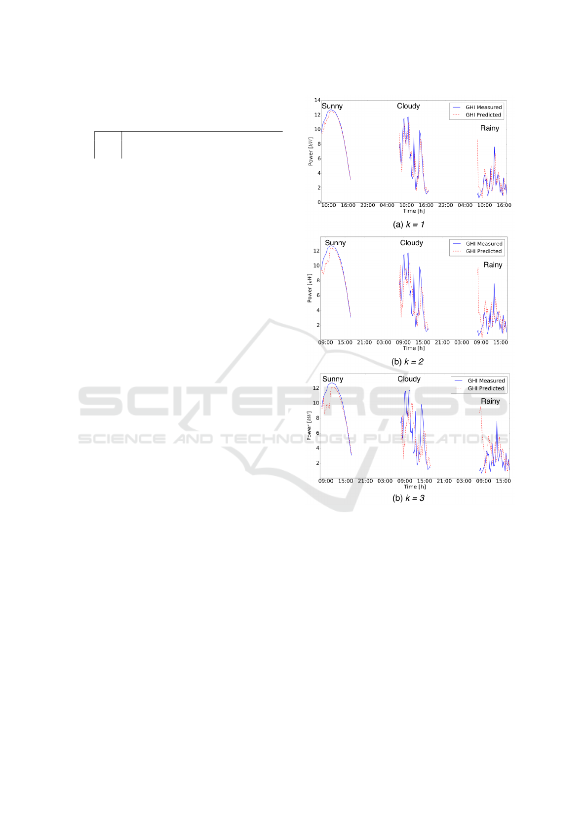
Table 2: Performance Indicator for PV simulation.

Time

[min]

MAD

[%]

MDB

[%]

RMSD

[%]

LCE WIA

k=1 15 11.33 -0.70 0.91 21.34 0.82 0.98

k=2 30 16.87 -0.81 0.84 28.81 0.73 0.96

k=3 45 20.97 -0.86 0.77 34.28 0.67 0.94

(see Section 4). Then, the PV simulator decomposes

GHI to estimate both Direct Normal Incident radia-

tion (DNI) and Diffuse Horizontal Incident radiation

(DHI) (Hoﬁerka and Ka

nuk, 2009). This decompo-

sition is done by exploiting state-of-the-art decom-

position models, such as (Engerer, 2015) and (Ruiz-

Arias et al., 2010), and considering the attenuation

caused by air pollution applying the Linke turbidity

coefﬁcient (Linke, 1922). Finally, the PV energy pro-

duction is given by applying the methodology presen-

ted in (Brihmat and Mekhtoub, 2014).

6.2 Results on PV Generation Forecast

In this section, we present the results of PV genera-

tion forecast in short-term time periods. In this scena-

rio, the PV simulator exploits GHI trends given by the

proposed neural network (see Section 4) with diffe-

rent time steps: i) k = 1 (i.e next 15 min.), ii) k = 2 (i.e

next 30 min.) and iii) k = 3 (i.e next 45 min.). To eva-

luate the errors of this approach, we repeated the PV

simulations with real GHI trends sampled by the we-

ather station in our campus. Fig. 6reports the plots of

the instant power for three generic days in June 2013:

i) sunny, ii) cloudy and iii) rainy. Generally, the trends

of our results with GHI forecast (dashed line) follow

with a good accuracy the behaviour of measured GHI

(continues line). As expected, simulations with k = 1

performs better than simulations with k = 2 and k = 3.

As shown in the three plots in Fig. 6, PV energy simu-

lations are more affected by errors during rainy days

especially during the early hours in the morning. This

is because the algorithm expects higher GHI values.

However, the algorithm is also able to recognize the

wrong GHI estimation and correct the error after few

time-steps.

Table 2 reports the performance indicators for si-

mulations with 1 ≤ k ≤ 3 with respect to simulati-

ons with sampled GHI trends. The performance in-

dicators show that increasing the predictive steps (k)

the accuracy on the results decreases. MAD increa-

ses from 11.33% for k = 1 to 20.97% for k = 3. Also

RMSD has a similar trend. r

for prediction step k = 1

is equal to 0.91. Whilst, the error increases with an

= 0.77 for k = 3. Finally, LCE varies from 0.82 to

0.67 and WIA decreases from 0.98 to 0.94.

These results conﬁrm that PV simulations with

GHI trends for 1 ≤ k ≤ 3 given by the proposed neu-

Figure 6: Simulations of PV energy production with k = 1

and k = 2 (June 2013).

ral network are acceptable to estimate the energy pro-

duction in the short-term time periods.

7 CONCLUSIONS

In this paper, we presented a methodology to forecast

the short-term solar radiation, suitable for photovol-

taic energy predictions. We discussed the results of

the neural network forecast, introducing the NAR ar-

chitecture able to base its prediction on a high number

of regressors. Furthermore, we compared our results

with real GHI values sampled by a real weather sta-

tion in our University campus. The analysis of per-

formance indicators highlighted an overall good per-

Forecasting Short-term Solar Radiation for Photovoltaic Energy Predictions

formance in predicting the solar radiation, especially

for the next 15, 30 and 45 minutes. As discussed, this

short-term forecast of solar radiation allows estima-

ting in advance the energy production of PV systems

with a good accuracy. This enables the design of more

accurate control policies for smart grids management,

such as Demand/Response.

ACKNOWLEDGEMENTS

This work was partially supported by the EU project

FLEXMETER and by the Italian project ”Ediﬁci a

Zero Consumo Energetico in Distretti Urbani Intel-

ligenti”.

REFERENCES

Aghaei, J. and Alizadeh, M.-I. (2013). Demand response

in smart electricity grids equipped with renewable

energy sources: A review. Renewable and Sustainable

Energy Reviews, 18:64–72.

Badescu, V. (2014). Modeling solar radiation at the earth’s

surface. Springer.

Bottaccioli, L., Estebsari, A., Patti, E., Pons, E., and Acqua-

viva, A. (2017a). A novel integrated real-time simu-

lation platform for assessing photovoltaic penetration

impacts in smart grids. Energy Procedia, 111:780–

789.

Bottaccioli, L., Patti, E., Macii, E., and Acquaviva, A.

(2017b). Gis-based software infrastructure to model

pv generation in ﬁne-grained spatio-temporal domain.

IEEE Systems Journal.

Box, G. E., Jenkins, G. M., Reinsel, G. C., and Ljung, G. M.

(2015). Time series analysis: forecasting and control.

John Wiley & Sons.

Brihmat, F. and Mekhtoub, S. (2014). Pv cell tempera-

ture/pv power output relationships homer methodo-

logy calculation. In International Journal of Scien-

tiﬁc Research & Engineering Technology, volume 1.

International Publisher &C. O.

Brockwell, P. J. and Davis, R. A. (2016). Introduction to

time series and forecasting. springer.

Chandrashekar, G. and Sahin, F. (2014). A survey on feature

selection methods. Computers & Electrical Engineer-

ing, 40(1):16–28.

Demuth, H. B., Beale, M. H., De Jess, O., and Hagan, M. T.

(2014). Neural network design. Martin Hagan.

Engerer, N. (2015). Minute resolution estimates of the dif-

fuse fraction of global irradiance for southeastern au-

stralia. Solar Energy, 116:215–237.

Gueymard, C. A. (2014). A review of validation methodo-

logies and statistical performance indicators for mo-

deled solar radiation data: Towards a better banka-

bility of solar projects. Renewable and Sustainable

Energy Reviews, 39:1024–1034.

Hamilton, J. D. (1994). Time series analysis, volume 2.

Princeton university press Princeton.

Han, S., Pool, J., Tran, J., and Dally, W. (2015). Learning

both weights and connections for efﬁcient neural net-

work. In Advances in Neural Information Processing

Systems, pages 1135–1143.

Hansen, L. K. et al. (1994). Controlled growth of cascade

correlation nets. In ICANN94, pages 797–800. Sprin-

ger.

He, X. and Asada, H. (1993). A new method for identifying

orders of input-output models for nonlinear dynamic

systems. In American Control Conference, 1993, pa-

ges 2520–2523. IEEE.

Hoﬁerka, J. and Ka

nuk, J. (2009). Assessment of photo-

voltaic potential in urban areas using open-source so-

lar radiation tools. Renewable Energy, 34(10):2206–

2214.

Kaplanis, S. and Kaplani, E. (2016). Stochastic prediction

of hourly global solar radiation proﬁles.

Kubat, M. (2017). Artiﬁcial neural networks. In An Intro-

duction to Machine Learning, pages 91–111. Sprin-

ger.

Legates, D. R. and McCabe, G. J. (2013). A reﬁned in-

dex of model performance: a rejoinder. International

Journal of Climatology, 33(4):1053–1056.

Linke, F. (1922). Transmissions-koefﬁzient und

ubungsfaktor. Beitr. Phys. Fr. Atmos, 10:91–103.

Ljung, L. (1998). System identiﬁcation. In Signal analysis

and prediction, pages 163–173. Springer.

Madanchi, A., Absalan, M., Lohmann, G., Anvari, M.,

and Tabar, M. R. R. (2017). Strong short-term non-

linearity of solar irradiance ﬂuctuations. Solar Energy,

144:1–9.

Miller, G. F., Todd, P. M., and Hegde, S. U. (1989). De-

signing neural networks using genetic algorithms. In

ICGA, volume 89, pages 379–384.

Montgomery, D. C., Jennings, C. L., and Kulahci, M.

(2015). Introduction to time series analysis and fo-

recasting. John Wiley & Sons.

Nazaripouya, H., Wang, B., Wang, Y., Chu, P., Pota, H.,

and Gadh, R. (2016). Univariate time series prediction

of solar power using a hybrid wavelet-arma-narx pre-

diction method. In Transmission and Distribution

Conference and Exposition (T&D), 2016 IEEE/PES,

pages 1–5. IEEE.

Norgaard, M., Ravn, O., and Poulsen, N. K. l. (2002).

Nnsysid-toolbox for system identiﬁcation with neural

networks. Mathematical and computer modelling of

dynamical systems, 8(1):1–20.

Norgaard, P. M., Ravn, O., Poulsen, N. K., and Hansen,

L. K. (2000). Neural networks for modelling and con-

trol of dynamic systems-a practitioner’s handbook.

Oancea, B. and Ciucu, S¸. C. (2014). Time series fo-

recasting using neural networks. arXiv preprint

arXiv:1401.1333.

Qazi, A., Fayaz, H., Wadi, A., Raj, R. G., Rahim, N., and

Khan, W. A. (2015). The artiﬁcial neural network for

solar radiation prediction and designing solar systems:

a systematic literature review. Journal of Cleaner Pro-

duction, 104:1–12.

SMARTGREENS 2018 - 7th International Conference on Smart Cities and Green ICT Systems

Rajamani, R. (1998). Observers for lipschitz nonlinear

systems. IEEE transactions on Automatic Control,

43(3):397–401.

Ruiz-Arias, J., Alsamamra, H., Tovar-Pescador, J., and

Pozo-Vzquez, D. (2010). Proposal of a regressive

model for the hourly diffuse solar radiation under all

sky conditions. Energy Conversion and Management,

51(5):881 – 893.

Siano, P. (2014). Demand response and smart gridsa survey.

Renewable and Sustainable Energy Reviews, 30:461–

478.

Siegelmann, H. T., Horne, B. G., and Giles, C. L. (1997).

Computational capabilities of recurrent narx neural

networks. IEEE Transactions on Systems, Man, and

Cybernetics, Part B (Cybernetics), 27(2):208–215.

Srivastava, N., Hinton, G. E., Krizhevsky, A., Sutskever, I.,

and Salakhutdinov, R. (2014). Dropout: a simple way

to prevent neural networks from overﬁtting. Journal

of machine learning research, 15(1):1929–1958.

Vardakas, J. S., Zorba, N., and Verikoukis, C. V. (2015). A

survey on demand response programs in smart grids:

Pricing methods and optimization algorithms. IEEE

Communications Surveys & Tutorials, 17(1):152–178.

Voyant, C., Darras, C., Muselli, M., Paoli, C., Nivet, M.-L.,

and Poggi, P. (2014). Bayesian rules and stochastic

models for high accuracy prediction of solar radiation.

Applied Energy, 114:218–226.

Voyant, C., Notton, G., Kalogirou, S., Nivet, M.-L., Paoli,

C., Motte, F., and Fouilloy, A. (2017). Machine le-

arning methods for solar radiation forecasting: A re-

view. Renewable Energy, 105:569–582.

Weather Underground. http://www.wunderground.com.

Willmott, C. J., Robeson, S. M., and Matsuura, K. (2012).

A reﬁned index of model performance. International

Journal of Climatology, 32(13):2088–2094.

Yadav, A. K. and Chandel, S. (2014). Solar radiation pre-

diction using artiﬁcial neural network techniques: A

review. Renewable and Sustainable Energy Reviews,

33:772–781.

Forecasting Short-term Solar Radiation for Photovoltaic Energy Predictions