Relative Pose Estimation in Binocular Vision for a Planar Scene using

Inter-Image Homographies

Marcus Valtonen

Ornhag and Anders Heyden

Centre for Mathematical Sciences, Lund University, Sweden

Keywords:

Relative Pose Estimation, SLAM, Visual Odometry, Binocular Vision, Planar Motion, Homography.

Abstract:

In this paper we consider a mobile platform with two cameras directed towards the ﬂoor mounted the same

distance from the ground, assuming planar motion and constant internal parameters. Earlier work related to

this speciﬁc problem geometry has been carried out for monocular systems, and the main contribution of this

paper is the generalization to a binocular system and the recovery of the relative translation and orientation

between the cameras. The method is based on previous work on monocular systems, using sequences of inter-

image homographies. Experiments are conducted using synthetic data, and the results demonstrate a robust

method for determining the relative parameters.

1 INTRODUCTION

In robotics research, it is of interest to accurately track

the position of a mobile robot relative to its surround-

ings. The emergence of artiﬁcial intelligence and au-

tonomous vehicles in recent years demand robust al-

gorithms to handle such problems. During the years

of research in the ﬁeld many kinds of sensors have

been used—LIDAR, rotary encoders, inertial sensors

and GPS, to mention a few—and often in combina-

tion. The type of sensor one chooses to work with re-

stricts what algorithms that can be used, and how the

resulting map of the robot and its surroundings will

look.

One sensor of particular interest for the robotics

and computer vision community is the image sensor

and there are many reasons why it is popular. One

important factor is that the wide range of algorithms

used in computer vision, e.g. visual feature extraction

and pose estimation, can be used in this setting; how-

ever, from an industrial point of view image sensors

are an often considered design choice since they are

relatively cheap compared to other sensors. Further-

more, they are often available on consumer products,

such as smartphones and tablets, where similar tech-

niques can be used, e.g. in Augmented Reality (AR).

With image sensors one is not limited to sparse 3D

clouds of feature points, but can model the map using

dense and textured 3D models.

Visual SLAM systems have been developed for

nearly three decades, with (Harris and Pike, 1988)

being one of the ﬁrst. Since then, several improve-

ments have been made, and with the aid of modern

computing power, a variety of methods for real-time

SLAM are available. Among the more recent once are

MonoSLAM (Davison et al., 2007), LSD-SLAM (En-

gel et al., 2014) and ORB-SLAM2 (Mur-Artal and

Tard

os, 2017), where the latter includes support for

monocular, stereo and RGB-D cameras.

2 RELATED WORK

In epipolar geometry, the fundamental matrix, intro-

duced by (Faugeras, 1992) and (Hartley, 1992), has

been a tool for many algorithms concerning scene

reconstruction; however, planar motion is known to

be ill-conditioned, see e.g. (Hartley and Zisserman,

2004). The problem geometry considered in this pa-

per is forced to planar motion, which is common in

e.g. indoor environments. To overcome this issue

algorithms that take advantage of planar homogra-

phies have been devised, which by construction are

constrained to planar motion and therefore do not

suffer from being ill-conditioned. Some early work

on planar motion using homographies include that

of (Liang and Pears, 2002) and (Hajjdiab and La-

gani

ere, 2004). More recent work on ego-motion re-

covery in a monocular system using inter-image ho-

mographies for a planar scene has been covered in

(Wadenb

ack and Heyden, 2013) for a single homogra-

568

Örnhag, M. and Heyden, A.

Relative Pose Estimation in Binocular Vision for a Planar Scene using Inter-Image Homographies.

DOI: 10.5220/0006695305680575

In Proceedings of the 7th International Conference on Pattern Recognition Applications and Methods (ICPRAM 2018), pages 568-575

ISBN: 978-989-758-276-9

phy and by the same authors for several homographies

in (Wadenb

ack and Heyden, 2014). In (Wadenb

ack

et al., 2017) the same methods are used to calibrate

the ﬁxed parameters initially, transforming the subse-

quent problem to a two-dimensional rigid body mo-

tion problem.

The stereo rig problem involving two cameras

with ﬁxed relative orientation is investigated for auto-

calibration in (Hartley and Zisserman, 2004). In (Ny-

man et al., 2010) a method for multi-camera plat-

form calibration using multi-linear constraints is de-

veloped; however, this method does not rely on the

inter-image homographies, but rather using the cam-

era matrices.

3 THEORY

3.1 Problem Geometry

In this paper we consider a mobile platform with two

cameras directed towards the ﬂoor mounted the same

distance from the ground. By a suitable choice of

the world coordinate system the cameras move in the

plane z = 0 and relative to the ground plane positioned

at z = 1. Both cameras are assumed to be mounted

rigidly onto the platform and no common scene point

is assumed to be visible in the cameras simultane-

ously. Furthermore, the mobile platform’s center of

rotation is assumed to be located in the ﬁrst camera

center. In this setting the second camera center is con-

nected to the ﬁrst by a rigid body motion.

The 3D rotations are parametrized using Tait-

Bryan angles

R(ψ,θ,ϕ) = R

(ψ)R

(θ)R

(ϕ), (1)

where R

, R

and R

denote the rotation around the

respective coordinate axes with a given angle. The

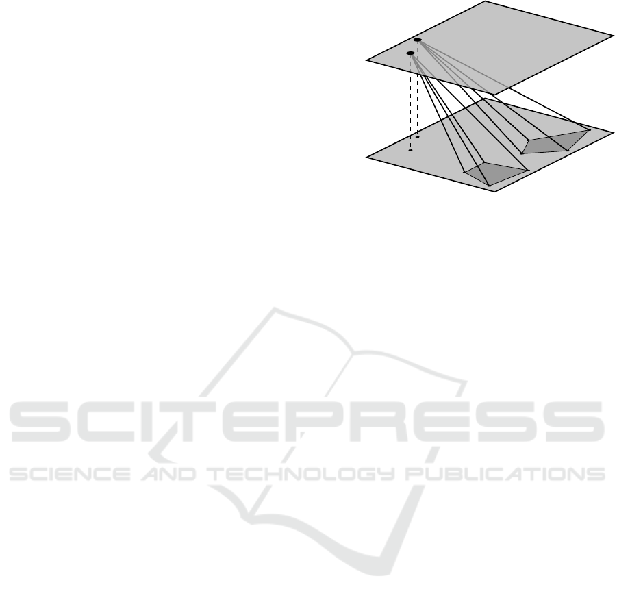
problem geometry is illustrated in Figure 1.

3.2 Camera Parametrization

As in (Wadenb

ack and Heyden, 2013), consider two

consecutive images, A and B, for the ﬁrst camera. The

camera matrices are then

= R

ψθ

I | 0

0],

= R

ψθ

I | − t

t],

(2)

where R

ψθ

is a rotation θ around the y-axis followed

by a rotation of ψ around the x-axis. The movement

of the mobile platform is modelled by a rotation ϕ

around the z-axis, corresponding to R

and translation

vector t

z = 1

plane normals

z = 0

Figure 1: The problem geometry considered in this paper.

The cameras are assumed to move in the plane z = 0 and

the relative orientation between them as well as the tilt to-

wards the ﬂoor normal is assumed to be ﬁxed as the mobile

platform moves freely.

The camera matrices for the second camera can be

parametrized as

= R

I | 0

0],

= R

I | − t

t],

(3)

where R

is the tilt, deﬁned as for the ﬁrst cam-

era. Furthermore, R

is a ﬁxed rotation by η degrees

around the z-axis relative to the ﬁrst camera, and τ

τ is

the rigid body translation vector between the ﬁrst and

the second camera center. The matrix T

corresponds

to a translation by τ

τ deﬁned as T

= I

I − τ

τn

, where

n = (0, 0, 1)

is a ﬂoor normal.

3.3 Homographies

Given point correspondences x

and x

, in homoge-

neous coordinates, the homography H

H transforms the

points such that x

= λH

, where λ 6= 0 is due to uni-

versal scale ambiguity. In (Wadenb

ack and Heyden,

2013) the homography for the ﬁrst camera is derived

and is given by

λH

H = R

ψθ

. (4)

Similarly, the homography H

for the second camera

is given by

= R

−1

. (5)

3.4 Parameter Recovery

By separating the ﬁxed angles from ϕ and the transla-

tion t

t the following relation holds

= λR

ψθ

= λ

−1

(6)

It is shown in (Wadenb

ack and Heyden, 2013) how

to recover the parameters for the monocular case, and

Relative Pose Estimation in Binocular Vision for a Planar Scene using Inter-Image Homographies

569

by doing so the parameters ψ, θ, ϕ and t

t aswell as ψ

and θ

can be recovered; the latter two from treating

the second camera as a monocular system. Further-

more, we shall assume that all homographies H

H are

normalized such that detH

H = 1.

3.4.1 Recovering the Relative Translation τ

The relative translation and rotation can be separated

by putting (3.4) in the form

−1

= λ

, (7)

and multiplying with the transpose from the left on

both sides yield

t−

−

−τ

t−

−

−τ

= λ

(8)

The left hand side of (3.4.1) can be simpliﬁed to

L =





1 0 `

0 1 `





, (9)

where

= τ

−t

− τ

sinϕ − τ

cosϕ,

= τ

−t

+ τ

sinϕ − τ

cosϕ,

= k

+ k

+ cτ

+ |t

+ 1,

(10)

and

= 2(t

cosϕ −t

sinϕ −t

= 2(t

sinϕ +t

cosϕ −t

c = 2(1 − cos ϕ) .

(11)

The eigenvalues of L are given by λ

= 1 and λ

, λ

such that λ

= `

− `

= 1. Furthermore, the

right hand side of (3.4.1) has the same eigenvalues

as H

, as they are similar. Since the sum of the

eigenvalues is the trace of the corresponding matrix,

the following relation holds

trH

= 2 + `

, (12)

which is independent of η. By letting h = tr H

H −

3 − |t

the relation becomes

+ k

+ cτ

− h = 0 . (13)

The other invariants do not give any new relations

for τ

τ since, det L = 1 and



(trL )

− trL



= trL .

3.4.2 Solving for the Relative Translation τ

With only one pair of homographies one cannot deter-

mine τ

τ explicitly; however, using multiple pairs one

equation on the form (13) for each pair of homogra-

phy is given, which yields a system of equations

(1)

+ k

(1)

+ c

(1)

(τ

+ τ

) − h

(1)

= 0,

(2)

+ k

(2)

+ c

(2)

(τ

+ τ

) − h

(2)

= 0,

(n)

+ k

(n)

+ c

(n)

(τ

+ τ

) − h

(n)

= 0 .

(14)

The system in (14) is over-determined for n > 2,

hence minimizing

min

τ∈

∑

i=1



(i)

+ k

(i)

+ c

(i)

(τ

+ τ

) − h

(i)



, (15)

gives the desired result. This can be re-formulated as

min

τ∈

Kτ

τ + c

cτ

τ − h

, (16)

where

K =







(1)

(2)

) k

(n)







, c

c =







(1)

(2)

(n)







and h

h =







(1)

(2)

(n)







(17)

By introducing a new variable r = |τ

τ|

, an equivalent

problem is obtained

min

τ∈

, r=|τ

τ|

Kτ

τ + c

cr − h

= min

x∈

, r=|τ

τ|

x − h

(18)

where x

x = (τ

, τ

, r)

and M

M = [K

K | c

c], where the

objective function can be written as

x − h

= x

x + d

x + h

h, (19)

where Q

Q = M

M and d

= −2h

M. In conclusion,

one may consider minimizing f (x

x) = x

x + d

subject to x

+ x

− x

= 0. Note that, the constraint

can be written as x

x + b

x = 0, where

A =









and b

b =





−1





. (20)

The Lagrangian is given by

L (x

x;λ) = x

x + d

x + λ(x

x + b

x), (21)

and solving ∇

L (x

x;λ) = 0

0 results in

x = −

Q + λA

−1

d + λb

b) . (22)

The constraint ∇

L (x

x;λ) = 0 yields a rational equa-

tion in λ, which can be turned into ﬁnding the roots of

a ﬁfth degree polynomial. This in turn can be trans-

lated into an eigenvalue problem, and solved robustly.

Using this approach solving (16) takes ∼100 µs which

is suitable for real-time applications. Furthermore,

due to the precision of modern eigenvalue solvers, the

error is usually negliable.

ICPRAM 2018 - 7th International Conference on Pattern Recognition Applications and Methods

570

3.4.3 Solving for the Relative Orientation η

Given τ

τ from the previous step consider (3.4) and

multiply the ﬁrst homography with the matrix corre-

sponding to the translation τ

τ. This yields

ψθ

−1

∼ R

, (23)

where η is the only unknown parameter. Deﬁne

W = T

ψθ

−1

and W

= R

and

note that W

W and W

share the same eigenvalues since

they are similar and the corresponding eigenvectors

are rotated η degrees.

Let us recall that the null space of a matrix is

spanned by the right-singular vectors corresponding

to zero—or due to noise, vanishing—singular val-

ues. Using the same approach as in (Wadenb

ack and

Heyden, 2014) we conclude that nulldimW

= 1.

Consequently, the eigenvectors spanning the null

spaces, x

x ∈ N (W

W ) and x

∈ N (W

), can be

obtained using SVD—this ensures that we work with

real eigenvectors.

We will use the following theorem to recover η

robustly, using all available pairs of homogaphies.

Theorem 1. Let Y

Y ,Y

∈

3×N

and non-zero. Fur-

thermore, let R

= R

(η) be a rotation matrix, cor-

responding to a rotation of angle η around the third

axis. Then

min

η∈(−π,π]

λ6=0

− λR

Y k

, (24)

is solved when

opt

= α +

(

0, if y

> 0,

π, otherwise,

(25)

where α may be expressed using the programming

friendly atan2 function,

α = atan2



− y

, y

+ y



. (26)

Here y

denotes the column vector of dimension N

corresponding to the i:th row of Y

Y . The vectors y

are

deﬁned analogously. The angles are considered as

equivalence classes, where η ≡ η + 2πk, k ∈ , with

the class representative being in the interval (−π,π].

Proof. Using the relation between the Frobenius

norm and the trace, the square of the objective func-

tion can be simpliﬁed

− λR

Y k

= tr



− λR

Y )(Y

− λR

Y )



= trY

− λ trY

− λ tr R

+ λ

trR

(27)

Since the trace is invariant under cyclic permutations

it follows that the last term is independent of η. Fur-

thermore,

trY

= tr









= tr R

. (28)

Combining these observations (24) is equivalent to

solving

min

η∈[−π,π)

λ6=0

Y k

− 2λtrR

. (29)

The reader can easily verify that the optimum is

reached when η is on the form (24).

In conclusion, the angle η may be obtained using

Theorem 1 where the i:th column of Y

Y corresponds to

the eigenvector spanning the null space of W

—

the matrix Y

is deﬁned analogously.

4 EXPERIMENTS

4.1 Synthetic Data

In order to validate the theory and evaluate the al-

gorithm synthetic data was generated in form of se-

quences of images mimicking those taken by a mo-

bile platform as described in Section 3.1. A high-

resolution image of a planar scene, in this case a tex-

tured ﬂoor, was chosen to yield many key-points. Fur-

thermore, different paths simulating the mobile plat-

form was deﬁned. In order to simulate the tilt the

original image was transformed around a given point

along the pre-deﬁned path and then cropped, such that

the center point in the cropped image coincide with

this point. The parameters used in the transforma-

tion serve as ground truth, and the resolution used in

each image is 400 × 400 pixels. The ﬁeld of view

of the simulated camera is normalized to 90 degrees,

which affects the impact of the distortion of the im-

ages caused by the cameras being tilted.

4.2 Homography Estimation

The homography estimation was done by extract-

ing SIFT keypoints (Lowe, 2004) from every frame,

keeping the most prominent once as candidates for

key-point matching. The remaining key-points are

then matched between subsequent images only, us-

ing a brute-force matcher based on the K Nearest

Neighbor algorithm. From the matched key-points a

random subset is chosen iteratively in the RANSAC

framework and from these a homography is esti-

mated. The homography with the highest amount of

Relative Pose Estimation in Binocular Vision for a Planar Scene using Inter-Image Homographies

571

Figure 2: Path of the simulated mobile platform for the ﬁrst camera (left) and the second camera (right). The red dots represent

the absolute position of the camera and the blue squares are the extracted images. The impact of the tilt is illustrated by the

frames not being square, but rather slanted. Note that the second camera path is not elliptic as the translational components

are affected by the rotation of the mobile platform.

inliers is chosen, where the maximum allowed repro-

jection error for a point pair to be considered as an

inlier is ﬁve pixels.

4.3 Parameter Recovery

4.3.1 Monocular Case

The parameters were recovered using the method pro-

posed in (Wadenb

ack and Heyden, 2014) for both tra-

jectories, treated as two independent monocular sys-

tems, using ﬁve homographies to determine the tilt,

rotation and translation in each step.

4.3.2 Recovering the Relative Translation

The optimal relative translation vector was obtained

by solving (16) using the optimization scheme pro-

posed in Section 3.4.2.

4.3.3 Recovering the Relative Orientation

Using the closed form solution presented in Theo-

rem 1 the relative rotation around the z-axis was es-

timated for the ﬁve pairs of homographies used in the

previous step. The computations involves ﬁnding the

vectors spanning the null spaces in order to compute

the matrices used in the closed form expression (24)

for η which is computationally inexpensive.

4.4 Test Cases

4.4.1 Elliptic Path

This case simulates the mobile platform moving in an

elliptic path while rotating between the images. The

test case was choosen as it includes general motions

which generates many different combinations of val-

ues for the nonﬁxed parameters. The sequence of

images for both cameras used in this case is shown

in Figure 2. The parameters used in this experi-

ment are ψ = 3.3

◦

, θ = −1.2

◦

, ψ

= 5.1

◦

, θ

= −4.6

◦

τ = (100, 80) and η = 30

◦

The results from analyzing the two paths indepen-

dently are shown in Figure 3 and the estimation of the

relative pose is shown in Figure 4.

4.4.2 Rotation Around the First Camera Center

Estimating the tilt in a monocular system with only

rotations and no translation is generally hard. A pos-

sible beneﬁt of a binocular system is that the rigid

body motion between the cameras results in a trans-

lational component in the second camera. The gen-

erated paths are shown in Figure 5. All ﬁxed angles

are set to 0

◦

and the relative translation τ

τ = (800, 0).

Furthermore, the mobile platform is moving with a

constant rotation.

ICPRAM 2018 - 7th International Conference on Pattern Recognition Applications and Methods

572

0 10 20 30 40 50

Homography number

2.3

2.8

3.3

3.8

4.3

ψ (de g rees)

0 10 20 30 40 50

Homography number

−2.2

−1.7

−1.2

−0.7

−0.2

θ (degrees)

0 10 20 30 40 50

Homography number

−30

−20

−10

ϕ (degrees)

0 10 20 30 40 50

Homography number

−5.0

−2.5

0.0

2.5

5.0

Error in t

and t

0 10 20 30 40 50

Homography number

4.1

4.6

5.1

5.6

6.1

′

(degrees)

0 10 20 30 40 50

Homography number

−5.6

−5.1

−4.6

−4.1

−3.6

′

(degrees)

0 10 20 30 40 50

Homography number

−30

−20

−10

ϕ (degrees)

0 10 20 30 40 50

Homography number

−5.0

−2.5

0.0

2.5

5.0

Error in t

and t

Figure 3: Estimated parameters for the ﬁrst camera (left) and the second camera (right). In all plots the blue circles represent

the ground truth. The red dots are the estimated parameters for the angles (ﬁrst three subplots) and in the last subplot the red

dots and the green diamond are the error in t

and t

respectively. The error in translation is measured in pixels. The estimates

have been calculated using ﬁve homographies at each frame.

0 10 20 30 40 50

Homography number

100

102

104

0 10 20 30 40 50

Homography number

0 10 20 30 40 50

Homography number

124

126

128

130

132

|τ |

0 10 20 30 40 50

Homography number

29.0

29.5

30.0

30.5

31.0

η (degrees)

Figure 4: Estimated value of τ

τ = (τ

, τ

) and η using ﬁve

pairs of homographies at each frame. The magnitude of the

translational component |τ

τ| is also shown. The red dots are

the estimated parameter and the blue circles represent the

ground truth.

Since (3.4.1) degenerates, as k

(i)

= k

(i)

= 0 for all

homographies, one cannot expect to recover the com-

ponents of τ

τ but it is possible to recover |τ

τ|, as shown

in Figure 6.

4.4.3 Mean Error vs. Number of Homographies

The relation between the accuracy and the amount

of homographies used to estimate the relative pose is

shown in Figure 7. The same setup as in Section 4.4.1

was used but the amount of homographies varied.

From the ﬁgures one can see that it is not a signiﬁcant

improvement in the parameter estimation of the rel-

ative pose after approximately twenty homographies.

In practice this means that the calibration could be

done initially, and then be used to track the position

of the mobile platform, without re-computation of the

ﬁxed parameters.

5 CONCLUSION

This paper has extended the work of (Wadenb

ack and

Heyden, 2014) to binocular vision. A method has

been deviced to robustly estimate the relative trans-

lation and orientation of the two cameras using sev-

eral pairs of homographies, by reusing the computa-

tions from the cameras treated as two monocular sys-

tems. The translational component is recovered by

solving a non-convex problem, which can be turned

into an eigenvalue problem. The proposed optimiza-

tion scheme is robust and suitable for real-time appli-

cations. Furthermore, when solving for the relative

Relative Pose Estimation in Binocular Vision for a Planar Scene using Inter-Image Homographies

573

Figure 5: Path of the simulated mobile platform for the ﬁrst camera (left) in the second test case, and for the second camera

(right). The red dots represent the absolute position of the camera and the blue squares are the extracted images. Due to

the rigid body motion connecting the cameras the second camera rotates around the ﬁrst camera center causing a non-zero

translational component.

0 10 20 30 40 50

Homography number

795.0

797.5

800.0

802.5

805.0

|τ |

Figure 6: Estimated value of |τ

τ| using ﬁve pairs of homo-

graphies at each frame. When considering only rotations

for the ﬁrst camera, the components of τ

τ cannot be obtained

by the proposed method. The red dots are the estimated pa-

rameter for the magnitude and the blue circles represent the

ground truth.

0.4

0.6

0.8

= kτ

− τ

∗

0 10 20 30 40 50

Number of homographies

0.10

0.15

= |η

− η

∗

Mean error

Figure 7: Mean error for the relative translation and rota-

tion as a function of the number of pairs of homographies

used in the optimization step. The error for the translational

component is measured in the Euclidean norm. The mean

error is computed from 49 pairs of homographies estimated

from the sequence described in Section 4.4.1.

rotation, the closed form solution presented in The-

orem 1 is computationally inexpensive. Experimen-

tal results from synthetic data have demonstrated that

the method has an acceptable accuracy for most prob-

lems, and highlighted problems where the method

fails to recover both of the translational components;

it is also shown that in this case the magnitude can be

recovered accurately.

ACKNOWLEDGEMENTS

This work has been funded by the Swedish Research

Council through grant no. 2015-05639 ‘Visual SLAM

based on Planar Homographies’.

REFERENCES

Davison, A. J., Reid, I. D., Molton, N. D., and Stasse, O.

(2007). Monoslam: Real-time single camera slam.

IEEE Transactions on Pattern Analysis and Machine

Intelligence, 29(6):1052–1067.

Engel, J., Sch

ops, T., and Cremers, D. (2014). LSD-

SLAM: Large-Scale Direct Monocular SLAM, pages

834–849. Springer International Publishing, Cham.

Faugeras, O. D. (1992). What can be seen in three di-

mensions with an uncalibrated stereo rig. In Pro-

ceedings of the Second European Conference on Com-

puter Vision, ECCV ’92, pages 563–578, London,

UK. Springer-Verlag.

Hajjdiab, H. and Lagani

ere, R. (2004). Vision-based multi-

robot simultaneous localization and mapping. In

Computer and Robot Vision, 2004. Proceedings. First

Canadian Conference on, pages 155–162. IEEE.

Harris, C. and Pike, J. (1988). 3d positional integration

from image sequences. Image and Vision Computing,

6(2):87 – 90.

ICPRAM 2018 - 7th International Conference on Pattern Recognition Applications and Methods

574

Hartley, R. and Zisserman, A. (2004). Multiple View Geom-

etry in Computer Vision. Cambridge University Press,

second edition.

Hartley, R. I. (1992). Estimation of relative camera po-

sitions for uncalibrated cameras, pages 579–587.

Springer Berlin Heidelberg, Berlin, Heidelberg.

Liang, B. and Pears, N. (2002). Visual navigation using

planar homographies. In ICRA ’02: Proceedings of

the 2002 IEEE International Conference on Robotics

and Automation, pages 205 – 210.

Lowe, D. G. (2004). Distinctive image features from scale-

invariant keypoints. International Journal of Com-

puter Vision, 60(2):91–110.

Mur-Artal, R. and Tard

os, J. D. (2017). Orb-slam2:

An open-source slam system for monocular, stereo,

and rgb-d cameras. IEEE Transactions on Robotics,

33(5):1255–1262.

Nyman, P., Heyden, A., and

Astr

om, K. (2010). Multi-

camera platform calibration using multi-linear con-

straints. 2010 20th International Conference on Pat-

tern Recognition, Pattern Recognition (ICPR), 2010

20th International Conference on, page 53.

Wadenb

ack, M. and Heyden, A. (2013). Planar motion

and hand-eye calibration using inter-image homogra-

phies from a planar scene. In 8th International Joint

Conference on Computer Vision, Imaging and Com-

puter Graphics Theory and Applications (VISIGRAPP

2013), Proceedings of, pages 164–168.

Wadenb

ack, M. and Heyden, A. (2014). Ego-motion recov-

ery and robust tilt estimation for planar motion using

several homographies. In Proceedings of the 9th Inter-

national Conference on Computer Vision Theory and

Applications (VISAPP 2014), pages 635–639.

Wadenb

ack, M., Karlsson, M., Heyden, A., Robertsson, A.,

and Johansson, R. (2017). Visual odometry from two

point correspondences and initial automatic tilt cali-

bration. In 12th International Joint Conference on

Computer Vision, Imaging and Computer Graphics

Theory and Applications (VISIGRAPP 2017), pages

340–346.

Relative Pose Estimation in Binocular Vision for a Planar Scene using Inter-Image Homographies

575