Improving Range Prediction of Battery Electric Vehicles by Periodical
Calculation of Driver Parameters based on Real Driving Data
Kurt Kruppok
1
, Tobias Walter
1
, Reiner Kriesten
1
and Eric Sax
2
1
Institute of Energy Efficient Mobility (IEEM), University of Applied Sciences, Moltkestr. 30, Karlsruhe, Germany
2
Institute for Information Processing Technologies (ITIV), Karlsruher Institute of Technology (KIT),
Engesserstr. 5, Karlsruhe, Germany
Keywords:
Electric Vehicle, Driver Behaviour Prediction, Energy Demand Estimation, Driver Properties.
Abstract:
Due to the battery’s limited storage capacity, it is important to reduce energy consumption of electric vehicles.
Depending on the average speed, an aggressive driving behaviour can result in an up to 40% higher energy
consumption compared to an economic one. In this work, we propose a methodology, which calculates driver
parameters based on measured real drive speed and acceleration profiles as well as signposted speed limits. The
presented approach compares the energy consumption and driver parameters between our past estimation and
the real drive speed profile in order to continuously improve the energy demand estimation for the remaining
distance. Thus, this paper provides a procedure to increase the accuracy of energy demand estimation for
battery electric vehicles which helps to reduce the range anxiety. In future work, it will be used within a
navigation assistance system that supports the driver in reaching his destination with a low battery charge.
1 INTRODUCTION
Electrification of vehicles plays a major role in the
current change of the automotive industry. Particu-
larly, in case of battery electric vehicles (BEV), pre-
cise prediction of the available range is essential in
order to give the driver confidence in his vehicle. Fur-
thermore, it is necessary to determine wheater the des-
tination is reachable with the available energy or not.
In addition to the battery’s limited storage capac-
ity, the utilized range is even smaller due to the psy-
chological factor of range anxiety. This is the driver’s
fear not be able to continue driving because the bat-
tery is out of charge. In this case, it is - different to a
vehicle with combustion engine - not possible to get
a BEV ready to drive again with a few liters of fuel.
Due to this point and the small number of charging
stations, this fear is even higher compared to vehicles
with an internal combustion engine. The range anxi-
ety can be minimized by an accurate range prediction.
One factor that can significantly increase or re-
duce the vehicle’s range is the driving behaviour
(Badin et al., 2013). In addition to environmental
and traffic influences, the driving behaviour has to be
taken into account, in order to make the most accurate
energy demand estimation as possible. For this pur-
pose, the current behaviour has to be recognized and
included into the energy demand estimation.
These issues are addressed through the following
contributions:
• An approach to describe the driver’s behaviour
through a specific set of parameters without the
usual classification of the driver.
• A sensitivity analysis of the parameter set to in-
vestigate the influence of an individual parameter
on the energy demand for a given route.
• A methodology for evaluating the differences be-
tween current and predicted driving style and a
periodical adjustment of the relevant parameters
to increase prediction accuracy for the remaining
journey.
These points are described within the structure of this
paper as followed: In Sect. 2, we summarize previous
work concerning driver parameters as well as energy
demand estimation and distinguish our approach from
the state of the art. In Sect. 3, we explain the neces-
sary basics for understanding our energy demand es-
timation model, followed by a description of the cho-
sen driver parameter and their impact on the energy
demand in Sect. 4. Our proposed methodology is de-
scriped in Sect. 5 and subsequently, we discuss the re-
sults. In the last section, we summarise our outcomes
and describe further work.
Kruppok, K., Walter, T., Kr iesten, R. and Sax, E.
Improving Range Prediction of Battery Electric Vehicles by Periodical Calculation of Driver Parameters based on Real Driving Data.
DOI: 10.5220/0006696103490356
In Proceedings of the 4th International Conference on Vehicle Technology and Intelligent Transport Systems (VEHITS 2018), pages 349-356
ISBN: 978-989-758-293-6
Copyright
c
 2019 by SCITEPRESS – Science and Technology Publications, Lda. All rights reserved
349

2 RELATED WORK
In related work, driver types are usually divided into
different numbers of classes. For example, into the -
most commonly used - three classes relaxed, normal
and dynamic (Wilde et al., 2008; Park et al., 2017) or
into five classes aggressive, sporty, moderate, anxious
and energy efficient (B
¨
ar et al., 2011; Ara
´
ujo et al.,
2012).
A driver type is primarily definied by the aver-
age acceleration. For urban areas for example, de-
fined ranges are: calm 0.45 to 0.65 m/s
2
, normal 0.65
to 0.80 m/s
2
and aggressive driver 0.85 to 1.10 m/s
2
(de Vlieger et al., 2000). For motorways, on the
other hand, the acceleration for all three driver types
is only in the range from 0.08 to 0.20m/s
2
(Langari
and Won, 2005). Most of the related work use fuzzy
logic to classify the driver (B
¨
ar et al., 2011; Langari
and Won, 2005). A further approach is to use the ra-
tio of the standard deviation of the acceleration and
the average acceleration in order to get a better com-
parability (Langari and Won, 2005).
In this paper, we do not separate the driver
into predefined groups nor we evaluate his driv-
ing behaviour with a fuzzy set. This is one of
the main differences between this work and the
above-mentioned works. After the classification into
driver types, the properties are no longer modified.
Assuming that a driver is assigned to a specific
group of drivers, but his driving style changes within
the boundaries of the group, these changes are not
transferred to a subsequent prediction. This would
lead to an error in the energy demand estimation.
This error can be avoided by evaluating driving
data such as speed and acceleration during the jour-
ney rather than dividing it into individual driver types.
Another difference between this and related work
is the use of input quantities. Other work use the brake
pressure (B
¨
ar et al., 2011) or the moving average val-
ues of the gas and brake pedal during acceleration or
deceleration respectively (Wilde et al., 2008). Spa-
tial (speed limits, roundabouts, school zones, ...) and
temporal (purposes, time, day of the week, ...) condi-
tions are used by (Ellison et al., 2015). Mostly, the in-
put quantities are referenced to special situations such
as approaching towns and villages, taking sharp turns
and approaching a stop sign (B
¨
ar et al., 2011) or to
the driving environment (city, rural, motorway) based
on signposted speed limits (Castignani et al., 2013).
A further approach is to calculate the driver pa-
rameters through speed, acceleration and rotation rate
of a smartphone by processing the data from accelera-
tion sensor, magnetic field and GPS receiver (Castig-
nani et al., 2013; Ara
´
ujo et al., 2012).
In our work, we use a combination of speed limits
and the measured speed profile in order to calculate
driver-specific parameters, which form the base for
a new energy demand estimation. In contrast to a
classified type of driver, this allows us to measure the
driver characteristics depending on each speed limit
range. This avoids the mentioned problem of driving
style changes within the borders of a classified driver
type. Thus, we want to reduce the error in our energy
demand estimation.
A further distinguishing feature between this and
related work is the processing of the collected data.
We continuously calculate parameters which serve for
the determination of cornering speed, acceleration,
braking and the resulting upper speed limit. More-
over, the real and simulated energy consumption are
compared in order to determine correction factors,
which then influences the renewed estimation through
feedback. From all above-mentioned works, only
(Langari and Won, 2005) optimize the driver param-
eters by a direct comparison between estimation and
simulation.
Other work, for example, do not aim to use the
collected data for an energy demand estimation in a
closed-loop, rather they score the driver between 0
and 100, to evaluate the driving behaviour in terms
of accident risks and their avoidance (Ellison et al.,
2015) or in terms of cost-efficiency (Castignani et al.,
2013).
While recording trip data, our model distinguishes
whether a vehicle in front is present or not. This dis-
tinction results in two datasets of driver parameters,
with and without a vehicle in front. If the driver slows
down due to a vehicle in front, signal processing is
interrupted to avoid incorrect classification. This
approach has been partially adopted from (Wilde
et al., 2008) in this paper. The advantage of this is
that, depending on the predicted traffic volume, a
distinction can be made between whether the driver
has nearly unrestricted driving or the traffic is largely
determining his driving behaviour.
Within the framework of the presented methodol-
ogy, the results of the energy demand estimation are
applied as an input quantity. Other work that deals
with prediction of expected energy demand and range
estimation (Sehab et al., 2011; Vaz et al., 2015; Fer-
reira et al., 2013; Zhang et al., 2012), are not de-
scribed in detail here.
VEHITS 2018 - 4th International Conference on Vehicle Technology and Intelligent Transport Systems
350

3 ENERGY DEMAND MODEL
Our prediction model generates the forthcoming route
including environmental and traffic parameters. Then,
we calculate an estimated driving profile for this given
route on the basis of vehicle and driver parameters.
The individual steps are explained in the following
subchapters.
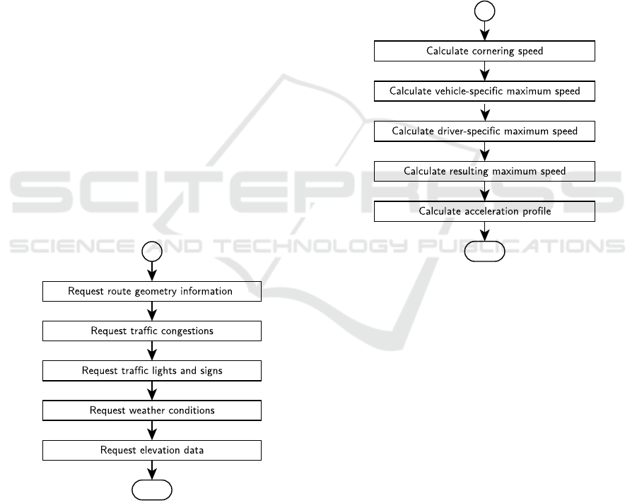
3.1 Generation of Route Data
In order to generate a virtual route, serveral data are
collected. Therefore, the route generating algorithm
runs through five steps shown in Fig. 1.
First, waypoints - which have a distance of about
100 meters to each other - are queried between start,
destination and optionally specified intermediate des-
tinations. Using these waypoints, different APIs re-
trieve traffic information (Step 2), route properties
(Step 3) such as speed limits, traffic lights, signs or
tunnels, and weather conditions (Step 4) along the
route. In the last step, the elevation data for each
waypoint of the generated route is determined by the
SRTM C-band dataset.
The necessary input data for the algorithm are:
• Starting point [LAT/LON]
• Destination [LAT/LON]
• Time [DD.MM.YYYY HH:MM]
Figure 1: Flow chart of route generating algorithm. The
input data are starting point, destination, time and optionally
one or more waypoints (Gutenkunst et al., 2015).
Subsequently, three postprocessing steps of the col-
lected data are executed:
• Transformation of coordinates [X,Y,Z]
• Calculation of slope [
◦
and α]
• Calculation of curve radius [m]
After completing the route generation and postpro-
cessing steps, a virtual route is available for further
use. Detailed information about the route generat-
ing algorithm and the subsequent postprocessing are
described in (Gutenkunst et al., 2015) and (Kruppok
et al., 2017), respectively.
3.2 Calculation of Vehicle Motion
The calculation of the vehicle’s motion profile is
based on the generated route data, descriped in the
previous subchapter. The five steps are shown in
Fig. 2.
Figure 2: Determination of vehicle motion profile based on
algorithm described in (Kruppok et al., 2017).
At first, the maximum lateral acceleration is used
to calculate the maximum cornering speed. Subse-
quently, the course of the resulting maximum speed
v
max
(lidcurve) is generated, which is the minimum
of the driver-specific maximum cornering speed, the
driver- and vehicle-specific maximum longitudinal
speed, the signposted speed limits and the deviation
to speed limits caused by driver’s behaviour. In the
last step, the driver parameters are used to calculate
the acceleration profile. The finally used accelera-
tion value for every single acceleration phase is de-
termined randomly within a normal distribution. The
average longitudinal acceleration is assumed to be the
expected value of the Gaussian function (Kruppok
et al., 2017).
3.3 Calculation of Energy Consumption
Based on the estimated driving profile and vehicle
parameters, the driving resistance equations (Eq. 2)
Improving Range Prediction of Battery Electric Vehicles by Periodical Calculation of Driver Parameters based on Real Driving Data
351

which include air F
drag
, rolling F
roll
, gradient F
grad
and acceleration resistance F
acc
are used to calculate
energy demand estimation E
Drive
, see Eq. 1.
E
Drive
= (F
roll
+ F
drag
+ F
grad
+ F
acc
) · s (1)
with
F
drag
=
c
d
· A · ρ · v
2
2
F
roll
= m · g · cos α
grad
· f
R
F
grad
= m · g · sin α
grad
F
acc
= m · a
F
(2)
4 DRIVER PARAMETERS
This section describes the driver parameters used in
the energy demand estimation model and shows a sen-
sitivity analysis to investigate their impact on the en-
ergy consumption. The analysis reveals the most in-
fluential parameters which are then used within the
presented methodology.
4.1 Applied Driver Parameters
Contrary to previous work, the driver is described by
the following six characteristics which influence the
energy demand estimation. The first three factors af-
fect the calculated upper speed limit (lidcurve). The
last three factors determine the acceleration and de-
celeration of the estimated speed profile:
• Maximum Lateral Acceleration (a
x
) is used to
calculate the maximum cornering speed.
• Global Speed Limit (v
drivermax
) represents the
driver’s desire of an upper speed limit. Usually, it
only has an effect on road sections without sign-
posted speed limits.
• Speed Limit Compliance (compliance
v
) is a
measure of the driver’s compliance with sign-
posted speed limits and has a major impact on all
groups of speed limits.
• Acceleration Behavior (scaling
a
) is greater than
1, if the driver accelerates or brakes rather
strongly, and less than one, if he accelerates or
brakes with restraint.
• Maximum Longitudinal Acceleration (a
x
) rep-
resents how dynamic the driving behaviour in
curves is.
• Maximum Longitudinal Deceleration (a
brake
)
describes the intensity of the driver’s braking pro-
cedures. The minimum value and the default
value can be identical, if the vehicle determines
the deceleration due to the recuperation mode,
which is active when the accelerator pedal is
pressed slightly or not at all.
4.2 Sensitivity Analysis
In order to investigate the influence of driver parame-
ters on the energy consumption, a sensitivity analysis
with the six parameters mentioned above is carried
out. In each case, the same route with the same vehi-
cle and environmental conditions is simulated, so that
only the driver parameters are varied. The total en-
ergy consumption and the share caused by air resis-
tance are calculated from the varied driving profiles.
The analysis is based on recorded GPS tracks of a
BMW i3, but is equally applicable for other BEVs.
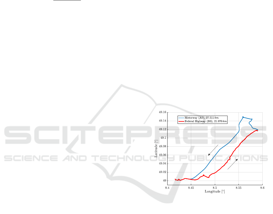
The way from Bruchsal to Karlsruhe and back is
used for the analysis and has a overall distance of
49.481km, see Fig. 3. The outward route runs along
the motorway (A5) with a length of 27.511 km, while
the return route is 21.970 km long and follows a fed-
eral highway (B3).
Figure 3: Route with color-separated outward and return
path used for sensitivity analysis and algorithm validation.
Each parameter set is simulated several times,
since the acceleration within the energy demand es-
timation model is determined by a random Gaussian
distribution. From these simulations, the mean value
is calculated to minimize the random error and to
make the results more comparable. By simulating
with different parameter sets, the effect of a single
factor on energy consumption is shown. Therefore,
adjustments can be implemented more effectively.
Initial values, step size and range of variiation are
shown in Table 1.
The results of the analyis in Table 2 show that
compliance
v
and scaling
a
have the largest impact on
the total energy demand.
VEHITS 2018 - 4th International Conference on Vehicle Technology and Intelligent Transport Systems
352

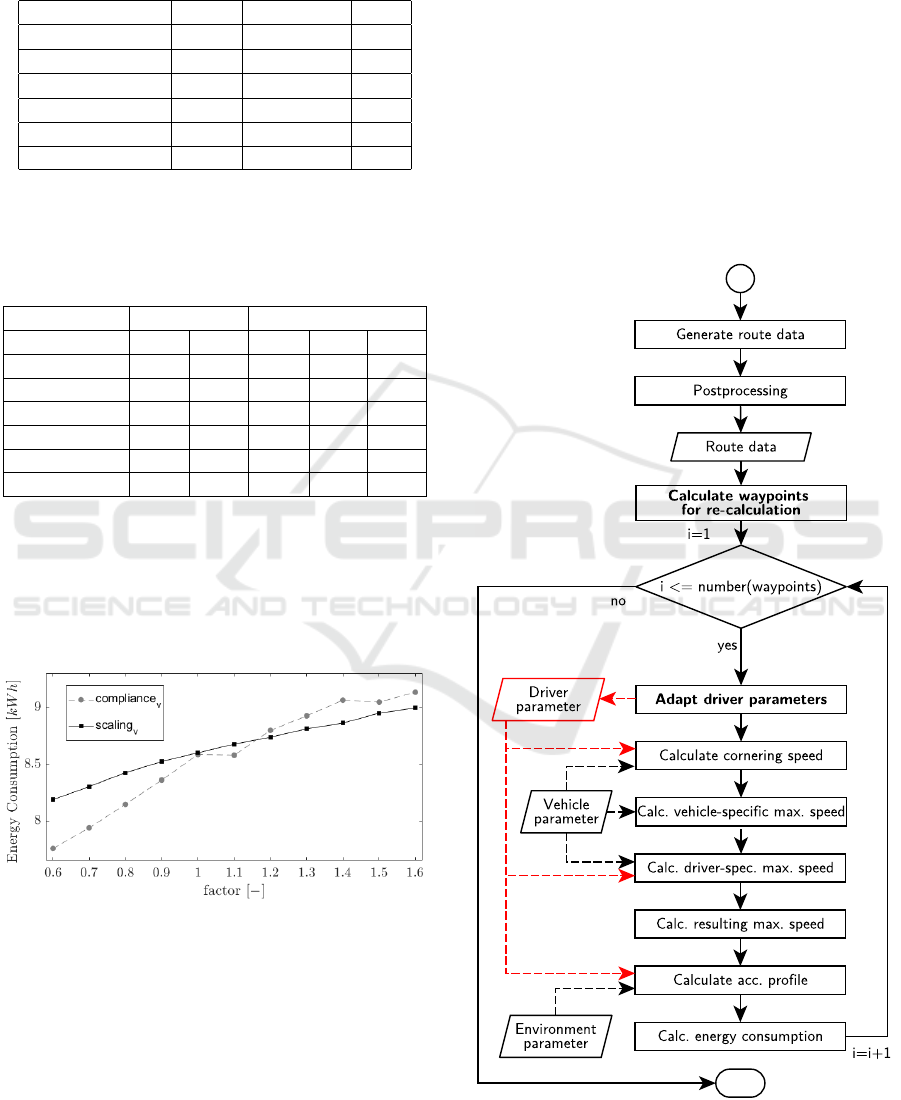
Table 1: Overview of the six driver parameters and their
initial value, step size and their range of variiation within
the sensitivity analysis procedure. The step size has been
selected to obtain arround 10 values for each parameter.
Parameter Initial Range Step
a
x
[m/s
2
] 3 3 to 7 0.5
a
brake
[m/s
2
] -1.6 -2 to -1 0.1
a
y
[m/s
2
] 5 0.5 to 5.5 0.5
v
drivermax
[km/h] 130 125 to 150 2.5
compliance
v
[−] 1 0.6 to 1.6 0.1
scaling
a
[−] 1 0.6 to 1.6 0.1
Table 2: Results of the sensitivity analysis sorted in de-
scending order according to the largest energy difference:
Necessary maximum and minimum energy [kW h] to over-
come the air resistance and the overall driving resistances
depending on the varied six driver parameters.
Resistance Air Total
Max Min Max Min ∆
compliance
v
4.41 3.53 9.13 7.76 1.37
scaling
a
4.18 3.90 8.99 8.19 0.80
v
drivermax
4.51 3.91 9.16 8.43 0.73
a
y
4.08 3.73 8.65 8.15 0.50
a
brake
4.10 3.99 8.71 8.41 0.30
a
x
4.08 4.00 8.61 8.45 0.16
Thus, the following methodology uses these pa-
rameters for the periodical estimation of the energy
demand in order to adapt it to the real consumption.
The variation of these two factors between 0.6 and 1.6
as well as the resulting energy demand are shown in
Fig. 4.
Figure 4: Energy consumption for the variation of the driver
parameters scaling
a
and compliance
v
between 0.6 and 1.6
with a step size of 0.1.
The influence of v
Max
grows with the number of
sections without speed limitation along the route. In
addition, the lower v
Max
is defined, the more sections
are affected and the greater is the impact of this pa-
rameter. A change in longitudinal and lateral acceler-
ation has hardly any effect on energy consumption.
Only when the lateral acceleration falls below
1.5m/s
2
, it becomes relevant, due to the fact that the
resulting cornering speed is often lower than the sign-
posted speed limits. This results in a reduction of the
speed level and thus also of the necessary energy de-
mand. The lower the maximum longitudinal acceler-
ation, the more often the applied acceleration of the
driver model, which is based on a Gaussian distribu-
tion, is limited by this threshold value and the lower
is the energy demand.
5 METHODOLOGY
The data used for the investigation are based on a pre-
diction model on the one hand and on a real test drive
Figure 5: Flowchart of the main algorithm. The red arrow
indicates the usage of driver parameters. Bold text indicates
a new functions within the framework of our methodology.
Improving Range Prediction of Battery Electric Vehicles by Periodical Calculation of Driver Parameters based on Real Driving Data
353

on the other. Based on the parameter influences and
the existing speed profile calculation, the concept was
designed, see Fig. 5.
Subsequent to the RouteGeneration and Postpro-
cessing steps, mentioned in Sect. 3, the number of
waypoints at which the driver parameters are to be
recalculated is determined. Since the driver parame-
ters have no influence on the previous calculations for
determining the slope, curve radius and route geome-
try, they will not be updated periodically but rather
assumed to be static during the initial calculation.
This minimizes additional computing time. The way-
points required for the simulation, at which the re-
calculation of the parameters takes place, are time-
dependent and therefore not equidistant due to differ-
ent route courses. The period of time between way-
points can be variably selected in the model and is
limited only by the calculation time of the program
sequence.
The measured data are not used to classify the
driver. Instead, the above-mentioned parameters are
calculated from the data and these are directly in-
cluded in the simulation. In addition, a compar-
ison is made between the real and simulated en-
ergy consumption, in order to adjust the simula-
tion by means of the correction factors scaling
a
and
compliance
v
. The model derives driver parameters
from the recorded measurement data at several way-
points along the route. A simulation is carried out
periodicly at each individual waypoint.
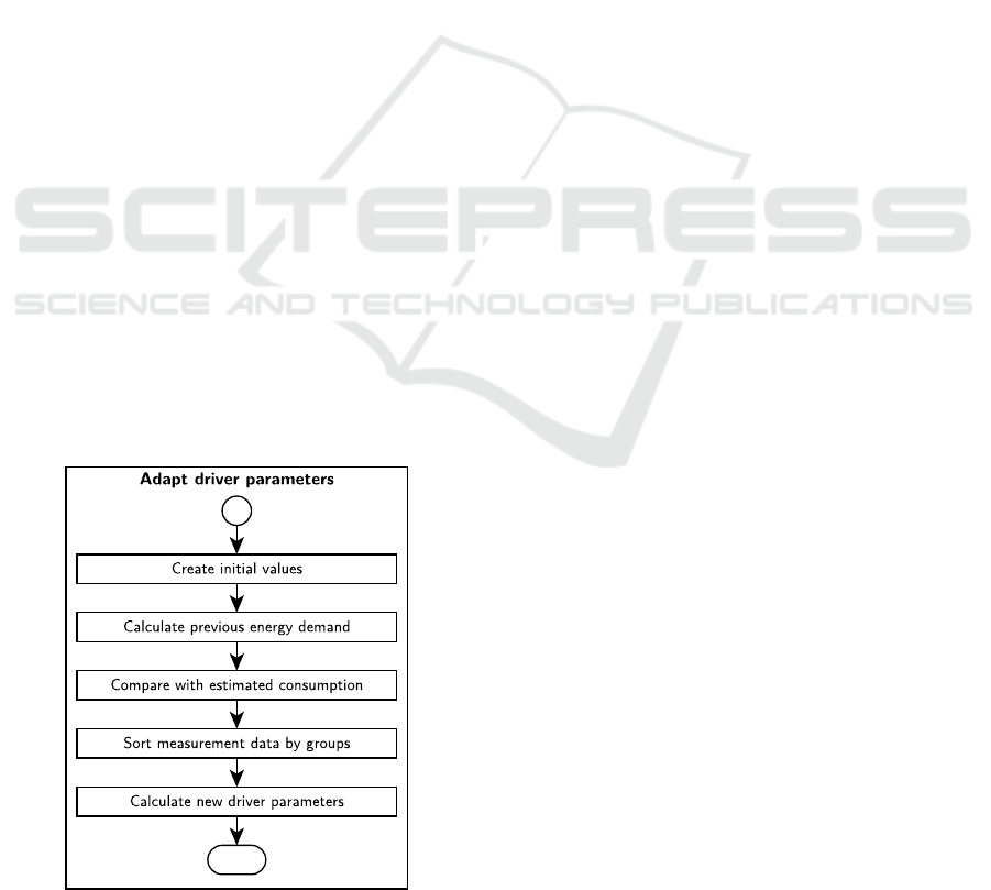
5.1 Adaptation of Driver Parameters
The driver parameters are determined step by step
from the measured data. The program’s simplified
flow chart is shown in Fig. 6.
Figure 6: Algorithm for adapting the driver parameters.
For the first prediction, the program uses initial
driver parameters. These are initially independent of
the current driver and his driving style, as there is no
data available on his upcoming driving behaviour. A
parameter set from past journeys, which can be as-
signed to a certain driver, for example by the iden-
tification with a unique key (of the vehicle or a car-
sharing ID) or by the selection of a certain seat po-
sition from the memory are conceivable, but do not
matter in the context of this paper.
Within the second iteration, which means the first
new prediction, measurement data have already been
collected and sorted according to various criteria. A
distinction is made between speed limits and whether
the test vehicle was preceded by a vehicle in front. For
sorting the speed limits, two approaches were com-
pared: a division of the measurement data into twelve
speed limit groups, from 30 km/h to 130 km/h in in-
crements of 10 km/h including a group for sections
without speed limits, as well as a division into three
speed limit groups. In the latter case, they are set to
slower than 60 km/h, 60 km/h to 100 km/h and faster
than 100 km/h. Accordingly, the last group contains
the sections without speed limit.
In addition to sorting measured data, the energy
consumption for the travelled distance so far is also
calculated, which then is used for a comparison with
the simulated energy consumption. Afterwards, the
sorted measurement data according to the driving sit-
uation are evaluated and, if possible, the correction
factors are determined. The factor scaling
a
, which
should correct the accelerations, is calculated by com-
paring the acceleration resistance energies. The cor-
rection factor compliance
v
, which represents the de-
viation to speed limits caused by driver’s behaviour,
results from a comparison of the air resistance energy.
6 RESULTS
The validation of our methodology is based on sim-
ulations with twelve and with three groups of speed
ranges, but it is conducted on the same route with the
same measurement data. Comparing the results of the
simulations with the real drive shows that both esti-
mated energy consumptions are too low, see Table 3.
The estimated energy consumption with twelve
and three speed range groups is 15% and 12 % lower,
respectivly, than the real energy consumption. The
differences of the energy of rolling resistance, gradi-
ent resistance and air resistance between simulation
and real driving are very small. A negligible differ-
ence in rolling resistance is due to inaccuracies in our
model for energy demand estimation compared to re-
VEHITS 2018 - 4th International Conference on Vehicle Technology and Intelligent Transport Systems
354

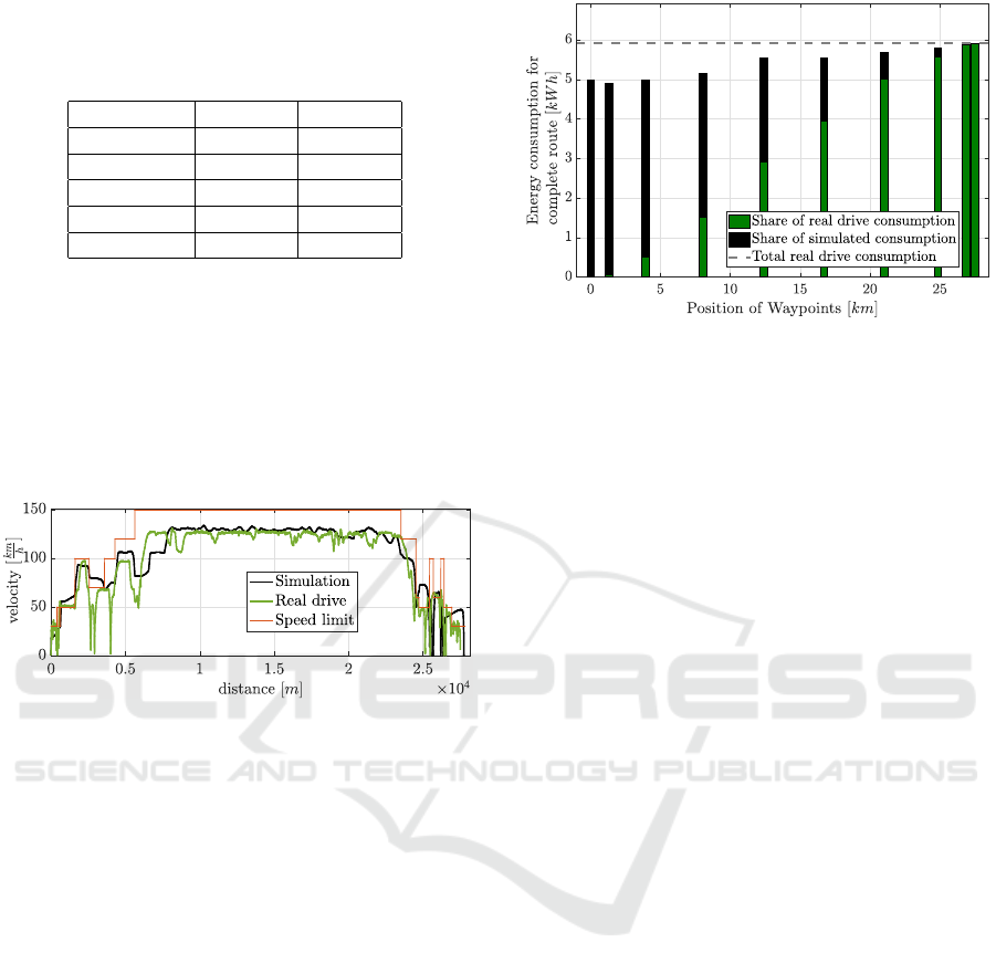
Table 3: Energy demand between simulation with twelve
and three speed groups compared to the real drive. All val-
ues given in the table are expressed relativ to the real drive
energy consumption.
# of groups twelve three
E
drag
3.5% 5.3 %
E
roll
0.9% 0.9 %
E
acc
−44.2% −40.3 %
E
grad
0.0% 0.0 %
E
total
−14.9% −12.0 %
ality.
The decisive difference is caused by the accel-
eration resistance. The deviation of our estimation
compared to the real drive values can partly be ex-
plained by significant differences in the speed profile,
see Fig. 7. These represent a journey from Bruchsal
to Karlsruhe via the A5 motorway, whose course is
already presented in Fig. 3.
Figure 7: Speed limitation and speed profiles from simula-
tion and real drive.
Due to red traffic lights at the beginning of the real
journey, the vehicle slowed down three times from ar-
round 70km/h - twice even to a complete standstill -
and accelerated back to the initial speed. These de-
celeration and acceleration phases do not take place
in the simulation, as the status of the traffic lights has
been randomly determined. In addition, the speed
fluctuations on the section without speed limit are
more pronounced in reality than in simulation, which
also contribute a small part to the energy difference.
For this reason, it can be seen that from the next way-
point after the 10km mark, there is a significant in-
crease in accuracy regarding the estimation of the to-
tal energy demand, see Fig. 8
7 CONCLUSIONS
This paper presented a methodology to adapt driver
paramters based on a measured speed profile in or-
der to improve the accuracy of the energy demand es-
timation for the upcoming route. At the beginning
of this paper, our model for energy demand estima-
tion was presented and a sensitivity analysis with the
Figure 8: Comparison of predictively determined and real
energy consumption. At each waypoint, energy consump-
tion for the entire route is calculated from previous real
drive and remaining energy demand estimation.
driver-specific parameters was carried out. The effect
of individual driver parameters on the result of the es-
timation was determined and it was found that large
deviations can be caused by the scaling of the over-
all acceleration behaviour and the non-observance of
speed limits.
Subsequently, a function was introduced which
determines these driver parameters on the basis of
measured real drive data. The route was divided into
several waypoints. On each point, the previous mea-
surement data since the start of the journey are used to
derive the driver’s characteristics. This data is used on
every single waypoint for a new energy demand esti-
mation. The results have shown that a significant de-
viation occurs due to route-dependent circumstances.
Grouping the driver parameter on the basis of differ-
ent speed ranges revealed that 12 groups do not offer
an advantage compared to 3 groups.
Further work will cover real driving data including
the information about a vehicle in front. It is planned
to use the traffic volume as a distinguishing feature in-
stead of the division between with/without a vehicle
in front, e. g. in the gradation none, light, medium and
heavy. In addition, the classification of speed classes
into groups of different sizes is also investigated in
order to achieve an optimum between the number of
data points per group and the accuracy of the driv-
ing behaviour. Further investigations will show which
distances between the periodical predictions are nec-
essary and whether the consideration of the route pro-
file brings added value to the determination of these
distances. Furthermore, we will investigate whether
time-weighted pedal signals, as they are also used by
(Wilde et al., 2008), result in a more precise estima-
tion, i. e. whether newer signals have a higher influ-
ence than older ones.
Improving Range Prediction of Battery Electric Vehicles by Periodical Calculation of Driver Parameters based on Real Driving Data
355

REFERENCES
Ara
´
ujo, R., Igreja,
ˆ
A., de Castro, R., and Araujo, R. E., edi-
tors (2012). Driving coach: A smartphone application
to evaluate driving efficient patterns. IEEE.
Badin, F., Le Berr, F., Briki, H., Dabadie, J. C., Petit, M.,
Magand, S., and Condemine, E., editors (2013). Eval-
uation of EVs energy consumption influencing factors,
driving conditions, auxiliaries use, driver’s aggres-
siveness. IEEE.
B
¨
ar, T., Nienh
¨
user, D., Kohlhaas, R., and Z
¨
ollner, J. M., ed-
itors (2011). Probabilistic driving style determination
by means of a situation based analysis of the vehicle
data. IEEE.
Castignani, G., Frank, R., and Engel, T. (2013). Driver
behavior profiling using smartphones. 16th Interna-
tional IEEE Conference on Intelligent Transportation
Systems (ITSC 2013), pages 552–557.
de Vlieger, I., de Keukeleere, D., and Kretzschmar, J. G.
(2000). Environmental effects of driving behaviour
and congestion related to passenger cars. Atmospheric
Environment, 34(27):4649–4655.
Ellison, A. B., Greaves, S. P., and Bliemer, M. C.
(2015). Driver behaviour profiles for road safety anal-
ysis. Accident Analysis & Prevention, 76(Supplement
C):118–132.
Ferreira, J. C., Monteiro, V., and Afonso, J. L., editors
(2013). Dynamic range prediction for an electric ve-
hicle. IEEE.
Gutenkunst, C., Chrenko, D., Kriesten, R., Neugebauer,
P., J
¨
ager, B., and Giereth, T. (2015). Route gener-
ating algorithm based on opensource data to predict
the energy consumption of different vehicles. In Vehi-
cle Power and Propulsion Conference (VPPC), 2015
IEEE.
Kruppok, K., Gutenkunst, C., Kriesten, R., and Sax, E.
(2017). Prediction of energy consumption for an au-
tomatic ancillary unit regulation. In Bargende, M.,
Reuss, H.-C., and Wiedemann, J., editors, 17. Interna-
tionales Stuttgarter Symposium, Proceedings, pages
41–56. Springer Fachmedien Wiesbaden, Wiesbaden
and s.l.
Langari, R. and Won, J.-S. (2005). Intelligent energy man-
agement agent for a parallel hybrid vehicle-part i: Sys-
tem architecture and design of the driving situation
identification process. IEEE Transactions on Vehic-
ular Technology, 54(3):925–934.
Park, K., Son, H., Bae, K., Kim, Y., Kim, H., Yun, J., and
Kim, H. (2017). Optimal control of plug-in hybrid
electric vehicle based on pontryagin’s minimum prin-
ciple considering driver’s characteristic. Proceedings
of the 3rd International Conference on Vehicle Tech-
nology and Intelligent Transport Systems - Volume 1:
VEHITS, pages 151–156.
Sehab, R., Barbedette, B., and Chauvin, M., editors (2011).
Electric vehicle drivetrain: Sizing and validation us-
ing general and particular mission profiles. IEEE.
Vaz, W., Nandi, A. K. R., Landers, R. G., and Koylu, U. O.
(2015). Electric vehicle range prediction for constant
speed trip using multi-objective optimization. Journal
of Power Sources, 275:435–446.
Wilde, A., Schneider, J., and Herzog, H.-G. (2008). Driv-
ing situation and driving style dependent charging
strategy in hybrid electric vehicles. ATZ worldwide,
110(5):18–24.
Zhang, Y., Wang, W., Kobayashi, Y., and Shirai, K., editors
(2012). Remaining driving range estimation of elec-
tric vehicle. IEEE.
VEHITS 2018 - 4th International Conference on Vehicle Technology and Intelligent Transport Systems
356