Power and Cost-aware Virtual Machine Placement in
Geo-distributed Data Centers
Soha Rawas, Ahmed Zekri, Ali El Zaart
Department of Mathematics & Computer Science, Beirut Arab University, Lebanon
Keywords: Carbon Footprint, Energy-efficient, Latency, Geo-distributed Data Centres.
Abstract: The proliferation of cloud computing due to its attracting on-demand services leads to the establishment of
geo-distributed data centers (DCs) with thousands of computing and storage nodes. Consequently, many
challenges exist for cloud providers to run such an environment. One important challenge is to minimize
cloud users’ network latency while accessing services from the DCs. The other is to decrease the DCs’
energy consumption that contributes to high operational cost rates, low profits for cloud providers, and high
carbon non-environment friendly emissions. In this paper, we studied the problem of virtual machine
placement that results in less energy consumption, less CO2 emission, and less access latency towards large-
scale cloud providers operational cost minimization. The problem was formulated as multi-objective
function and an intelligent machine-learning model constructed to improve the performance of the proposed
model. To evaluate the proposed model, extensive simulation is conducted using the CloudSim simulator.
The simulation results reveal the effectiveness of PCVM model compared to other competing virtual
machine placement methods in terms of network latency, energy consumption, CO2 emission and
operational cost minimization.
1 INTRODUCTION
Cloud computing is growing in popularity among
computing paradigms for its appealing property of
considering “Everything as a Service”.
Consequently, this led to a radical increase in the
data centres’ energy consumption, turning it into
high operational cost rates, low profits for Cloud
providers, and high carbon non-environment
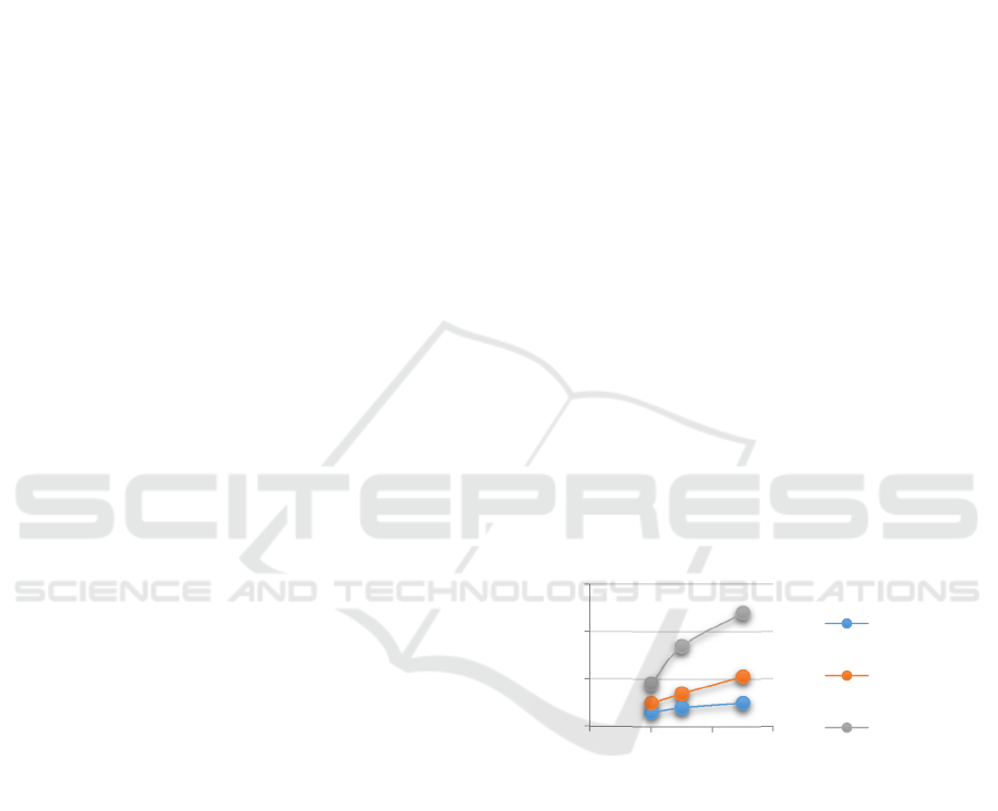
friendly emissions (Al-Dulaimy et al., 2016). Figure
1 displays the Synapse Energy Economics CO2
price/Ton forecast that will be applied all over the
world by the beginning of 2020 (Luckow et al.,
2016). Moreover, increasing awareness about CO2
emissions leads to a greater demand for cleaner
products and services. Thus, many companies have
started to build “green” DCs, i.e. DCs with on-site
renewable power plants to reduce the CO2 emission
which leads to operational cost minimization (Rawas
et al., 2015).
An important fact is that the carbon emission rate
varies from one DC to another based on the different
energy sources used to power-on the cloud DC
resources (such as coal, oil, and other renewable and
non-renewable resources) (Khosravi et al., 2013).
Figure 1: 2016 CO2 Price/Ton forecast by Synapse.
Moreover, the CO2 emission of DC is closely
related to electricity cost paid by cloud provider
since it depends on the sources used to produce
electricity (Fan et al., 2016). Therefore, selecting a
proper data centre for customer’s requests
dispatching attract research attention and have
become an emergent issue for modern geo-
distributed cloud DCs in big data era.
The modern geo-distributed data centres
proposed as a new platform idea are interconnected
with cloud users via the Internet. One of the most
challenging problems for this environment is
network latency when serving user request. Studies
0
50
100
150
2000 2020 2040 2060
Year
Low case ($)
Med case ($)
High case
($)
112
Rawas, S., Zekri, A. and El Zaart, A.
Power and Cost-aware Virtual Machine Placement in Geo-distributed Data Centers.
DOI: 10.5220/0006696201120123
In Proceedings of the 8th International Conference on Cloud Computing and Services Science (CLOSER 2018), pages 112-123
ISBN: 978-989-758-295-0
Copyright
c
2019 by SCITEPRESS – Science and Technology Publications, Lda. All rights reserved

show that minimizing latency leads to less
bandwidth consumption (Chen et al., 2013). This
consequently improves the provider revenue by
minimizing the Wide Area Network (WAN)
communication cost. Latency, which refers to the
time required to transfer the user request from user’s
end to the DC, is also taken into consideration for
Service Level Agreement (SLA) and Quality of
Service (QoS) purposes. Bauer et al. (Bauer et al.,
2012) show that Amazon Company can undergo 1%
sales reduction for a 100-millisecond increase in
service latency.
Inspired by the heterogeneity of DCs, carbon
emission rate and their modern geographical
distribution, this paper studies the virtual machine
(VM) placement and the physical machine selections
that result in less energy consumption, less CO2
emission, and less access latency while guaranteeing
the QoS. The main contributions of this study are as
follows:
1- Power and Cost-aware VM placement model
(PCVM) to beneficially affect the cloud user and the
cloud service provider.
2- Investigate the initial placement of offline and
online user request to enable the tradeoff among the
latency, energy consumption of the physical
machines, and the CO2 emission rate in geo-
distributed cloud DCs.
3- Intelligent machine-learning method to
improve the performance of the proposed PCVM
model
4- Comprehensive analysis and extensive
simulation to study the efficacy of the proposed
model using both synthetic and real DCs workload.
The rest of the paper is organized as follows:
Section 2 studies the related work concerning the
VM placement methods in geo-distributed data
centres. Section 3 presents the problem statement
and the proposed model. Section 4 presents the
proposed online and offline VM policies. Section 5
presents the performance metrics that have been
used to evaluate the proposed model. Section 6
models the intelligent machine-learning method for
normalized weight prediction. Section 7 presents the
evaluation method using CloudSim simulation
toolkit. Section 8 concludes the paper and presents
future work.
2 RELATED WORK
With the increase of distributed systems, the
problem of resource allocation attracted researchers
from its different views inspired by the
heterogeneity of the modern large-scale geo-
distributed data centres.
Khosravi et al. (Khosravi et al., 2013) propose a
VM placement algorithm in distributed DCs by
developing the Energy and Carbon-Efficient (ECE)
Cloud architecture. This architecture benefits from
distributed cloud data centres with different carbon
footprint rates, Power Usage Effectiveness (PUE)
value, and different physical servers’ proportional
power by placing VM requests in the best-suited DC
site and physical server. However, the ECE
placement method does not address the network
distance and considers that the distributed DCs are
located in the same USA region where the
communication latency and cost are negligible. Chen
et al. (Chen et al., 2013) modeled the VM placement
method in terms of electricity cost and WAN
communication cost incurred between the
communicated VMs. Ahvar et al. (Ahvar et al.,
2015) addressed the problem of DCs selection for
inter- communicated VMs to minimize the inter-
DCs communication cost. Malekimajd et al.
(Malekimajd et al., 2015) proposed an algorithm to
minimize the communication latency in geo-
distributed clouds. Jonardi et al. (Jonardi et al.,
2015) considered the time-of-use (TOU) electricity
prices and renewable energy sources when selecting
DCs. Fan et al. (Fan et al., 2016) modeled the VM
placement problem using the WAN latency,
network, and servers’ energy consumption factors.
The proposed model is different from the
aforementioned ones since it addresses the problem
of increase in CO2 emission and turning it into
operating cost. Moreover, the WAN network latency
factor is considered and formulated as an additional
operational cost.
3 SYSTEM MODEL
In this section, we describe PCVM, a Power and
Cost aware Virtual Machine placement model for
serving users’ request in geo-distributed cloud
environment. PCVM performs user request by
weighting each request’s effect on three important
metrics that increase the providers as well as the
cloud users cost: carbon emission rate, energy
consumption, and access latency.
3.1 Motivation and Typical Scenario
With more than 900 K servers, Google has 13 data
centres distributed within 13 countries around the
world (Google). While Amazon Application Web
Power and Cost-aware Virtual Machine Placement in Geo-distributed Data Centers
113
Services (AWS) has 42 data centres within 16
geographical regions with more than 1.3 million
servers (AWS, 2017). Consequently, the operating
cost has become a predominant factor to the cloud
services deployment cost.
The worldwide distribution of DCs provides the
fact that different geographical regions mean
different energy sources (coal, fuel, wind, solar
energy, etc.). DC’s CO2 emission rate depends on
the used electricity driven by these energy sources to
run the physical machines (Zhou et al., 2013).
Additionally, PUE can be considered as an effective
parameter to perform the VM placement. It indicates
the energy efficiency of the DC (Khosravi et al.,
2013). Proportional power of physical machines is
another important parameter. Selecting proper
physical machines to process user’s request has a
great impact on energy consumption (Al-Dulaimy et
al., 2016). Network latency and latency cost (lc)
have a great impact on cloud QoS and increases the
cloud provider operational cost.
Considering these important parameters, the
PCVM model aims to select the best suited DC site
and physical servers to increase the environmental
sustainability and minimize the cloud provider’s
operating cost.
3.2 Cloud Model Architecture
This section presents the cloud architecture model
that captures the relationship between cloud users
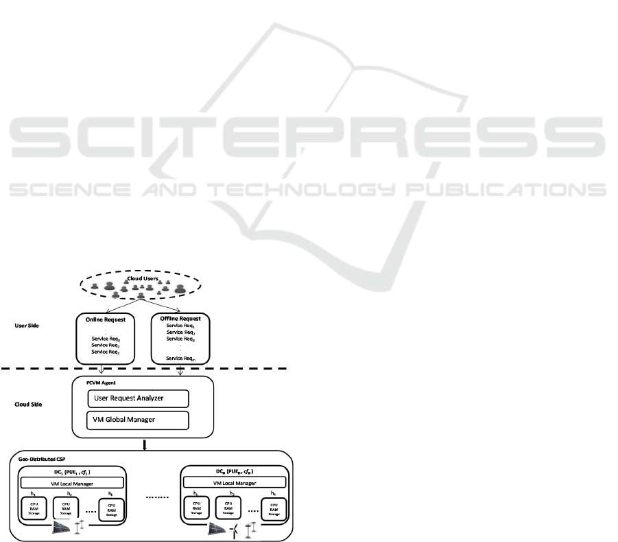
and geo-distributed cloud environment. Figure 2
encapsulates a simple abstract model representing
the relation between the following two main sides:
Users side and the Cloud side.
Figure 2: Cloud Model Architecture.
1- User Side: Cloud Users send their Service
Request to the Cloud side. The requested services
may be an application of any type such as: data
transmission (uploading or downloading), web
application, data or compute-intensive applications.
Cloud Users’ requests can be Online or Offline
Request. The Online Request is an expensive
Service Request with high priority. This type of
users’ request is processed by the Cloud
instantaneously. The Offline Request, on the other
hand, are handled as batches by the Cloud side.
2- Cloud Side: This side presents the cloud
infrastructure and it is made up of the following two
main sub components:
a- PCVM Agent: The PCVM is a cloud service
provider’s (CSP) broker that acts as an intermediary
between the cloud user and the CSP services. The
goal of this agent is to redirect the user request to the
nearest DC site that process requested services in a
greener and minimum operational cost without
scarifying cloud QoS. It contains the following sub
components:
• User Request Analyzer (URA): its functions are
- For each user’s Service Request (Req
i
), it allocates
the proper VM (VM
i
) to serve the cloud users.
- Interprets and analyzes the requirements of
submitted requested services (in terms of CPU,
RAM, Storage, Bandwidth …) to find the proper
VMs that serves the requested services.
- Finalizes the SLAs with specified prices and
penalties depending on user’s QoS requirements.
• VM Global Manager: Global cloud resources
manager
- Receives the set of VMs from URA. It interacts
with Geo-Distributed CSP VM Local Managers to
check each DC PUE, carbon footprint emission
rate (cf), and latency cost (lc) to take the best VM
placement decision on the DC site selection (lc
and cf illustrated in Sections 3.3.3 and 3.3.4
respectively).
- Observes energy consumption caused by VMs
placed on physical machines and provides this
information to the DC site VM Local Manager to
make optimization and energy-efficient
management decisions.
- Provides the VM Local Manager of the selected
DC site that should process the cloud user’s
request with the VM placement decision policy
(as proposed in Section 4).
b- Geo-Distributed CSP: A service provider has
geo-distributed DCs. Each DC has heterogeneous
computing and storage resources as well as different
utilities and energy sources. Each DC contains an
essential node called VM Local Manager. The VM
CLOSER 2018 - 8th International Conference on Cloud Computing and Services Science
114

Local Manager applies VM management and
resource allocation policies as suggested by the VM
Global Manager. Moreover, it calculates energy and
carbon emission rate of DC resources to provide this
information to the VM Global Manager.
3.3 Problem Formulation
Table 1 summarizes the various notations used in the
proposed VM placement problem formulation.
Table 1: Problem formulation notations.
Notation Description
D Number of DC sites
H Number of hosts at each DC
V
Total number of VMs on
host h
j
P
idle
Server power consumption
with no load
P
full
Fully utilized server power
consumption
U Amount of CPU utilization.
PUE
i
The power usage
effectiveness of DC site i
,
)
the unit transfer cost of
between DC site dc
i
and
cloud user u
e
; $/GB
,
)
the communication cost for
a flow size of data d
k
from
user u
e
served by DC site
dc
i
,
)
flow size of data d
k
from
user u
e
served by DC site
dc
i
Total CO2 emission cost; $
Total communication cost; $
CO2 emission cost per ton;
$/Ton
Total CO2 emission at a
time interval [0, T]; Ton
DC site i CO2 emission
rate; Ton/MWh
Users
Total number of users
requesting cloud services at
time t
data
Set of requested user’s
services data
,
)
is 1 if data d
k
is placed in server
hj in DC dc
i
; otherwise, it is 0;
Preliminaries
To model the VM placement method, a number of
factors are considered, these parameters
demonstrated as preliminaries before proceeding in
complete formulation.
3.3.1 Power Consumption Model
In this paper, the energy consumption and saving
predicted using the linear power model derived by
Fan et al. (Al-Dulaimy et al., 2016). A linear power
model verifies that the servers’ power consumption
is almost linearly with its CPU utilization. This
relationship could be illustrated using the following
equation:
)
=
−
∗ (1)
where P
idle
is server power consumption with no
load, P
full
is fully utilized server power consumption,
and u is the amount of CPU utilization.
Therefore, the power consumption of a
server/host hj holding a number of VMs v on data
centre site i during the slot time [0, T] is denoted
asPh
,
)
. Noting that each host can hold more
than one VM: h
,)
=
∑
VM
,,
and each VM is
executed at only one host such that:
∑∑
VM
,,
=1
,∀VM
3.3.2 Power Usage Effectiveness (PUE)
PUE is the most popular measure of data centre
energy efficiency. It was devised by the Green Grid
consortium (Fan et al., 2016). It is a metric used to
compares different DC designs in terms of electricity
consumption (Khosravi et al., 2013). The PUE of
DC i is calculated as follows:
=
(2)
where dc
TotalPowerConsumption, is the total
amount of energy consumed by DC facilities such
the cooling system, the IT equipment, lightning, etc.
The dc
ITDevicesPowerConsumption is the power
drawn due to IT devices equipment.
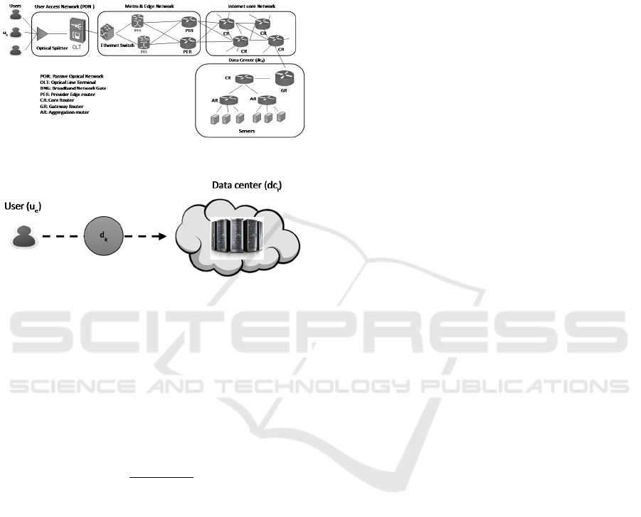
3.3.3 Network Model
Figure 3 shows the network model for the data
transmission between the cloud users who are
graphically at the same region, and the DC site
which is similar to the one presented in (Fan et al.,
2016). Therefore, we assume that each user ue is
connected by a WAN link. These links cost the
cloud provider whose bill is based on the actual
usage over a billing period (Chen et al., 2013). The
unit cost of data transfer between the DC site dci and
cloud user ue is denoted as UnitTransferCost(ue,dci)
in $/GB. However, the cost of intra-DC
communication is ignored since it is very low
compared with WAN transfer cost (Fan et al., 2016).
Power and Cost-aware Virtual Machine Placement in Geo-distributed Data Centers
115
Therefore, the communication cost for a flow size of
data dk (GB) from user ue served by DC site dci is
calculated as follows (see Figure 4):
,
)
=
,
)
∗
)
(3)
Figure 3: Users connected to DC through WAN.
Figure 4: User (u
e
) sends data (d
k
) to DC (dc
i
) Scheme.
3.3.4 Carbon Footprint Emission Rate (cf)
DC carbon footprint emission rate is measured in
g/kW. It depends on the DC energy sources and
electricity utilities. Therefore, the carbon footprint
emission rate of DC i operated using l number of
energy sources (such as, coal, gas, others) is
computed as follows (Zhou et al., 2013):
=
∑
,
∗
∑
,
(4)
where E
,
is the electricity generated by energy
source k (such as coal), and cr
is the carbon
emission rate of the used utility k.
3.3.5 Modeling of the Optimization Problem
The PCVM aim to minimize the total cost through
minimizing the weighted sum of the two main
objectives: carbon emission cost, and network
communication cost. Refers to the symbol
definitions in Table 1 and preliminaries model as
discussed in the previous sections (sections 3.4.1 –
3.4.4), the PCVM problem can be formulated as
follows:
∗
∗
)
(5)
= ∗
(6)
=
∑
∗
∗
∑
ℎ
,
(7)
=
∑∑ ∑
,
)
(8)
subject to:
∑∑
ℎ
,
=1,∀
(9)
∑∑
,
)
ℎ
,
)
(10)
∑∑
,
)
ℎ
,
)
(11)
∑∑
,
)
ℎ
,
)
(12)
Equation 5 presents the PCVM optimization model.
α
&α
are constant normalized weights used for
weighting the two sub-objectives such that α
α
=1 (Section 6 demonstrates how these weights
are calculated using an intelligent machine learning
model). Equation 6 shows that the total CO2
emission cost is equal to the CO2 unit emission cost
per ton multiplied by the total DCs’ CO2 emission
for time interval [0, T]. Equation 7 calculates the
total carbon footprint (CF) of cloud provider that
depends on a number of factors as illustrated above
(sections 3.3.1, 3.3.2, and 3.3.4) and presented in
(Khosravi et al., 2013). Equation 8 represents the
communication cost as illustrated in section 3.4.3.It
depends on users’ flow size as well as the unit cost
of data transfer from cloud users’ location to
selected DC’s site. Equation 9 mandates that a user
request is executed at only one DC. Equations (10,
11, 12) dictates that the resources requirements of
the mapped VMs on a physical server cannot exceed
the total capacity of the server.
4 PCVM HEURISTICS FOR VM
PLACEMENT
In this section, we propose two different versions of
placement policies for the PCVM agent:
Offline-PCVM VM placement: indicates offline
VM placement such that the requested services
requirements are prior known by the PCVM Global
Manager.
Online-PCVM VM placement: indicates online
and continuous VM placement during the run-time
of the DCs. The user’s requests are coming one by
one,
such that the PCVM Global Manager has no
prior information about the requested services
requirements.
CLOSER 2018 - 8th International Conference on Cloud Computing and Services Science
116

4.1 Offline MF-PCVM
Assume that D is the total number of DC sites and
each DC site has h number of servers, such that h
varies between DCs. At a certain time t, PCVM
agent tries to optimally place the user VMs. For the
offline cloud user’s requested services, we propose
the MF-PCVM VM placement algorithm (see
Algorithm 1 below). It is a greedy method that
selects a DC site with minimum communication
latency cost, minimum PUE and minimum CO2
emission rate. In addition, the algorithm tries to
minimize the number of selected active servers.
Algorithm 1: Most-Full Power and Cost-aware virtual
machine placement (MF-PCVM).
Input: DC sites D={dc
1
,dc
2
,…,dc
s
}
HostList at each DC site h={h
1
, h
2
, … h
h
}
Users request vmList V={vm
1
,vm
2
,…,vm
n
},
N
etwork latency cost matrix lc(u
e
,dc
j
)
Output: destination for requested V’s
Processing:
1: Get information from DCs VM Local Manager
2: Sort DC sites D in an ascending order of (1 ∗PUE
*
c
f
+2 ∗ lc)
3: Fed selected DC site VM Local Manager to apply
Most-Full VM placement Policy
4: Sort hostList h in an ascending order to its
Utilization
5: For each vm in vmList V do
6: While host h
j
has enough capacity to accommodate vm
u
7: set vm
u
at host h
j
8: End While
9: End For
The URA module in the PCVM agent receives
the users requests and produces the proper VMs; the
VM Global Manager utilizes the information given
by the CSPs VM Local Manager to take the best DC
site selection that has the minimum (α1 ∗PUE * cf
+α2 ∗lc) (line 2). Then, it feeds the selected DC site
VM Local Manager with Most-Full VM placement
policy decision. The VM Local Manager sorts the
host lists in an ascending order to its Utilization (line
4). If the selected host hj has enough resources for
VM accommodation (line 6-8), hj will be a
destination for vmu.
4.2 Online BF-PCVM
BF-PCVM method is also a greedy algorithm (see
Algorithm 2 below) that uses the Best Fit method for
VMs placement and servers selections after locating
DC sites with minimum communication latency
cost, PUE and CO2 emission rate (line 2).
Algorithm 2: Best-Fit Power and Cost-aware virtual
machine placement (BF-PCVM).
Input: DC sites D={dc
1
,dc
2
,…,dc
s
}
HostList at each DC site h={h
1
, h
2
, … h
h
}
Users request vmList V={vm
1
,vm
2
,…,vm
n
},
N
etwork latency cost matrix lc(u
e
,dc
j
)
Output: destination for requested V’s
Processing:
1: While vmList do
2: Get information from DCs VM Local Manager
3: Sort DC sites D in an ascending order of (1∗PUE
*
cf + 2 ∗ lc)
4
: Fed selected DC site VM Local Manager to apply
Best-Fit VM placement Policy
5
: Sort hostList h in an ascending order to its Availability
6: For each host in sorted hostList
7: if host h
j
is suitable for vm
u
8: set vm
u
at host h
j
9: End For
10: End While
We adapted the Best-Fit VM placement strategy
so that the VM Local Manager sorts the list of host
in an ascending order to its Availability (line 5). If
the selected host hj has enough resources for VM
accommodation (line 6-9), hj will be a destination
for vmu.
4.3 Online BF-SLA-PCVM
The aim of the BF-SLA-PCVM algorithm is to
provide a trade-off between SLA violations and
energy saving to minimize the penalties cost for
SLA violations per active host.
Algorithm 3: Best-Fit SLA violation, Power and Cost-
aware virtual machine placement (BF-SLA-PCVM).
Input: DC sites D={dc
1
,dc
2
,…,dc
s
}
HostList at each DC site h={h
1
, h
2
, … h
h
}
Users request vmList V={vm
1
,vm
2
,…,vm
n
},
N
etwork latency cost matrix lc(u
e
,dc
j
)
Output: destination for requested V’s
Processing:
1: While vmList do
2: Get information from DCs VM Local Manager
3: Sort DC sites D in an ascending order of (1 ∗PUE
*
cf + 2 ∗ lc)
4: Fed selected DC site VM Local Manager to apply
Best-Fit-SLA VM placement Policy
5: Sort hostList h in an ascending order to its Availability
6: For each host in sorted hostList
7: if host h
j
is suitable for vm
u
with x MIPS margin
8: set vm
u
at host h
j
9: End For
10: End While
As Algorithm 3 shows, the main difference
between BF-PCVM and BF-SLA-PCVM is that the
Power and Cost-aware Virtual Machine Placement in Geo-distributed Data Centers
117
algorithm will use a margin of x MIPS (line 7) that
minimizes the SLA violation penalties cost and
contributes to revenue maximization.
5 PERFORMANCE METRICS
This section presents the performance parameters
that will be used to measure the effectiveness of the
proposed PCVM model.
Makespan: Makespan indicates the finishing time of
the last task requested by cloud customer. It
represents the most popular optimization criteria that
reflect the cloud QoS.
=
∈
(13)
where f
t
denotes the finishing time of task t.
Active Servers (AS): Minimizing the number of
active servers by utilizing the activated ones is an
important criterion for cloud service providers. It
leads to maximum profit through serving cloud
user’s requests with minimum number of resources
without degrades the cloud QoS. AS counts the
number of active servers that used to complete a
bunch of task per time slot.
=
∑∑
ℎ
)
(14)
where Ah
ji
denotes the activated hosts in distributed
DC sites D.
SLAH: SLAH is the SLA violation per active host.
It is the percentage of time an active host
experiences 100 % utilization of CPU. The SLAH
can be calculated as follows (Khosravi et al., 2013):
=
∑
_
_
(15)
where h,_ℎ
, and _ℎ
is
the total number of hosts, the h
j
SLA violation time,
and active time respectively.
Electricity Cost: The Electricity Cost metric
calculates the average amount of electricity cost per
day. Equation 16 illustrates the calculation:
=
∑
∗
∗
(16)
where
,
,
is the electricity price, power
consumption and the PUE at DC i respectively.
Revenue: The Revenue metric calculates the
average profit per day. The cloud provider Revenue
per day calculated using the following equation:
= −
−
−
−
(17)
where Total Income is the VMs income.
,
,
calculate
d using Equations 16, 6, and 8 respectively.
The
calculated as follows:
= ∗ (18)
6 WEIGHT PREDICTION
MODEL
The normalized weights of Equation 5 are important
factors that contribute in finding an optimal solution
to the VM placement problem. While deciding
among the multiple normalized weights (α
&α
),
each one can be in conflict with the other. We
applied machine learning (ML) techniques to
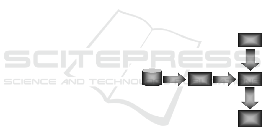
determine optimal values for the parameters. Figure
5 illustrates the basic schema of the proposed
methodology to find the PCVM-NWPM model. The
following sections describe the process of finding
the weights.
Figure 5: PCVM-NWP Model Scheme.
6.1 Phase 1
The first phase of the proposed prediction model
represents collecting the training data set to build the
ML model. The training set extracted according to
the probabilistic dependencies among PCVM
parameters. The structure of the data set parameters
are extracted knowledge and simulation results. For
forecasting of the input data, we use real DCs cloud
management information as represented in Table 2.
This information provides key insights to find the
important attributes that could affect the normalized
weights decision.
Training
Data Set
Train
ML Classifier
Algorithm
Create
PCVM-
NWPM
Online Data
Data
to
Predi
ct
Predi
cted
Data
Optimized
PCVM
Solution
CLOSER 2018 - 8th International Conference on Cloud Computing and Services Science
118

Table 2: Machine Learning Data Set Specifications.
Type Specifications
Workload 1-Planetlab (Planetlab
Traces, 2017)
2-Random Workload using
Uniform Distribution
Workload size (number of
tasks/per day)
1000-5000
VMs File Size (MB) 30-80
VMs EC2 (XSmall, Small,
Medium, Large)
PMs HP Proliant G4, G5
(Standard Performance
Evaluation Corporation,
2017)
Locations 3 different zones (Asia,
Europe, America)
Management System 1-MF-PCVM, BF-PCVM
& BF-SLA-PCVM
PUE 1.1-2.1 [Google Data
Centers, 2017, 30]
CO2 emission rate
(Ton/MWh)
0.1-0.7 (eia, 2017)
CO2 emission Cost
($/Ton)
20-120 (Luckow et al.,
2016)
WAN communication
Distance and Price ($/GB)
0.09 -0.25 (Fan et al., 2016)
6.2 Phase 2
In this phase, a classification algorithm is used to
learn the relationship between the training set
attributes collected at the first phase. To model a
finer predictor, we need to use a suitable ML
classifier with light computations. There are many
classification methods represented in literature such
as: Kernel Estimation, Decision Trees, Neural
Networks and Linear classifiers (Pereira et al.,
2009). However, when building an intelligent ML
predictor model, it is always important to take into
account the prediction accuracy. In that case, finding
the best algorithm to build our PCVM- NWPM
intelligent predictor depends on the accuracy and
reliability of the prediction model (Section 7.1.3
illustrates the used ML classifier type).
6.3 Phase 3
Using the learned PCVM-NWPM model, we are able
to predict the PCVM normalized weights. When VMs
request is made, the PCVM-NWPM intelligent predi-
ctor responsible of providing the normalized weights
of the PCVM objective function to execute the
requested VMs using the cost efficient DCs. It should
return the normalized weights that will provide the
optimum performance of the proposed PCVM model.
7 PERFORMANCE EVALUATION
To validate the effectiveness of the proposed model,
we have extended the CloudSim Toolkit to enable
PCVM VM placement policies testing. CloudSim is
an open source development toolkit that supports the
development of new management policies to
improve the cloud environment from its different
levels (Calheiros et al., 2011). To model the PCVM
VM placement methods, we utilized CloudSim 3.0.3
by modifying the DC broker algorithm that plays the
role of mediator between the cloud user and service
provider.
7.1 Simulation Setup
We conducted experiments on Intel(R) core(TM) i7
Processor 3.4GHz, Windows 7 platform using
NetBeans IDE 8.0.2 and JDK 1.8. Our simulation
has two different scenarios. Scenario1 is a synthetic
one that randomly modelled the cloud-computing
environment to measure the effectiveness of the
PCVM model in terms of AS and Makespan. In this
scenario, we modelled the offline IaaS environment
and applied the offline-PCVM approach. Scenario 2
modelled the online SaaS dynamic environment. It
applied the online-PCVM dynamic approach to
measure the efficacy of the proposed model with
respect to CO2 emission, Electricity Cost, Revenue
and more performance metrics as discussed in
section 5.
7.1.1 CO2 Emission Rate and PUR Data
To approximate the DC’s CO2 emission rate, we
used the information extracted from the U.S. Energy
Information website (eia, 2017). Its cost is taken as
20$/Ton as suggested by latest study of US
Government on CO2 emission economic damage
(Thang, 2015). While the PUE value for distributed
DCs is generated randomly in the range of [1.3, 1.8]
based on the Amazon and Google latest PUE
readings and work studied by Sverdlik (Google Data
Centers, 2017; Sverdlik, 2014).
7.1.2 Approximating Latency with Distance
Since there is no general analytical model for the
delay in the network, we use geographical distance
to approximate the network latency between a user
and geo-distributed DCs. Although distance is not an
ideal estimator for network latency, it is sufficient to
determine the relative rank in latency from end-user
to DCs as indicated in (Fan et al., 2016). Moreover,
Power and Cost-aware Virtual Machine Placement in Geo-distributed Data Centers
119

we use the WAN Latency Estimator (WAN Latency
Esitmator, 2017) to estimate the network latency in
milliseconds.
7.1.3 PCVM Normalized Weight Prediction
To model the PCVM-NWPM intelligent predictor,
we used the open source ML tool Weka (Hall et al.,
2009). Weka is an advanced tool designed by the
University of Waikato to provide data mining and
ML tasks. It contains a large number of ML
classifiers. We have tested several Weka’s embed-
ded ML algorithms to select an accurate predictor
model. The accuracy of the results was calculated
using the Mean Absolute Error (MAE) formula.
MAE is an ML classifier metric that measures the
average magnitude of the errors in a set of forecast.
Our training data set consisted of more than 4500
instances. 70% of data used as training set and the
rest used as testing set. In this paper, our approach
applies the machine learning k-nearest neighbor
technique (k-NN) (Weinberger et al., 2009) to the
workload data set to train the PCVM-NWPM model.
The k-NN method is a supervised learning algorithm
that helps to classify the ML data set in different
classes. It provides good prediction using a distance
metric.
7.2 Experimental Results
7.2.1 Scenario 1
To evaluate the Offline-PCVM policies, we
modelled an IaaS cloud environment with 4 DCs
sites (in 4 different geographical regions such as
USA, Europe, Brazil, and Asia). The aim of this
scenario is to strike a trade-off among the latency of
data access and the energy consumed by the DCs
that is evaluated using the workload Makespan and
AS metrics respectively.
Table 3 shows the relationship between DCs
distributed sites PUE, CO2 rate emission, number of
servers in each DC, and average distance between
the DCs sites and end users. Hosts are considered
homogenous of type HP ProLiant ML110 G5 (1 x
[Xeon 3075 2660 MHz, 2 cores], 4GB)
specifications to measure effectively the AS metric.
We assume that hosts will consume the full system
power when the server is on. We use small VM
instance type (1 EC2 Compute Unit, 1.7 GB),
inspired by Amazon EC2 instance type to run the
randomly generated bag-of-task workload. We use
SIGNIANT Flight pricing model as transferring
WAN pricing cost (Signiant, 2017).
Table 3: Geo-Distributed DCs Specifications.
DC dc1 dc2 dc3 dc4
PUE 1.3 1.7 1.65 1.5
CO2 Tons/MWh 0.864 0.350 0.466 0.678
Number of Hosts 900K 700K 500K 800K
Average Distance
(miles)
1000 1500 500 2000
Average Latency
(milliseconds)
21.35 30.23 12.48 39.1
WAN Transfer
Cost (S/GB)
0.087 0.138 0.087 0.181
Makespan. The algorithm used to compare the
Makespan metrics is MF-ECC. A Most full Energy
and Carbon-aware VM placement method and
similar version to MF-PCVM without considering
network latency for DC site selection. The objective
of this experiment is to find the effect of using
network latency as an important factor when
choosing DCs to execute users’ request.
Figure 6 shows the workload Makespan
improvement achieved by the location aware MF-
PCVM algorithm over MF-ECC method using 3
different numbers of VMs request as shown in Table
4. Taking the transferring cost into consideration,
our MF-PCVM algorithm significantly outperforms
the MF-ECC in achieving high cloud QoS with
approximate 25% rate of Makespan enhancement.
Table 4: Cloud Resources.
Simulation Type Number of VMs Number of
Cloudlets
Small 500 1000
Medium 1000 2000
Large 1500 3000
Figure 6: Workload Makespan in different number of
cloudlets and VMs.
AS. This experiment compares MF-PCVM with
Simple-PCVM. Simple-PCVM is similar version to
MF-PCVM in DCs selections; however, it chooses
the basic Simple method for host selection (the host
with less PEs in use).
0
100
200
300
400
500
Time in Seconds
Cloud Resources
Makespan
MF-PCVM
MF-ECC
CLOSER 2018 - 8th International Conference on Cloud Computing and Services Science
120
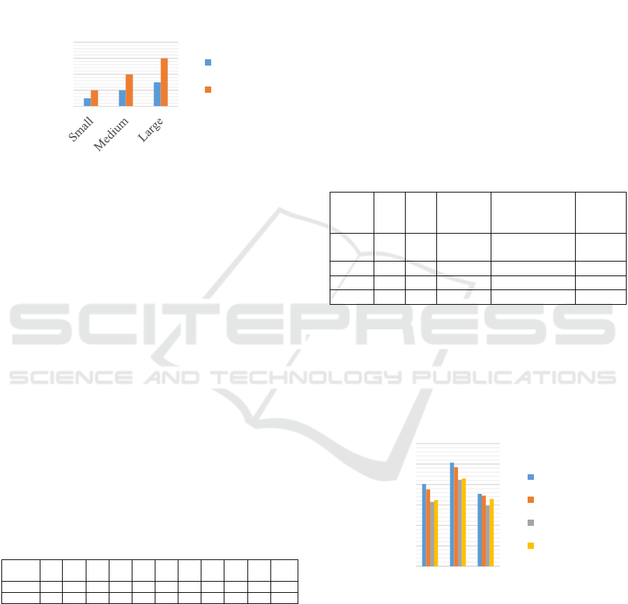
Figure 7 demonstrates that MF-PCVM VM
placement method reduces energy consumption with
an average of 50% compared to Simple-PCVM
algorithm and using 3 different numbers of VMs
request as shown in Table 4.. Note that, in this
experiment, the number of activated hosts is taken as
a measure for energy consumption.
Figure 7: AS in different number of cloudlets and VMs.
7.2.2 Scenario 2
This section evaluates the Online-PCVM proposed
policies. We employed real Planetlab traces to
emulate the online SaaS cloud environment. The
SaaS cloud environment was modelled with 4 DCs
sites. The DCs distributed sites PUE, CO2 rate
emission, and average distance between the DCs
sites and end users are the same as indicated in
Table 3. However, hosts are considered
heterogeneous of type HP ProLiant ML110 G4 (1 x
[Xeon 3040 1860 MHz, 2 cores], 4GB) & HP
ProLiant ML110 G5 (1 x [Xeon 3075 2660 MHz, 2
cores], 4GB) specifications. According to the linear
power model (Equation 1), and real data from
SPECpower benchmark (Standard Performance
Evaluation Corporation, 2017), Table 5 presents the
hosts power consumption at different load levels.
Table 5: HP servers host load to energy (Watt) mapping
table.
Server
type
0% 10% 20% 30% 40% 50% 60% 70% 80% 90% 100%
HP G4 86 89.4 92.6 96 99.5 102 106 108 112 114 117
HP G5 93.7 97 101 105 110 116 121 125 129 133 135
Four different VM types are used inspired by
Amazon EC2. Table 6 displays the characteristics of
VM instances and their hourly price. To generate a
dynamic workload, Planetlab benchmark workload
is employed to emulate the SaaS VM requests. Each
VM runs application with different workload traces.
Each trace is assigned to a VM instance in order. We
choose 3 different workload traces from different
days of the Planetlab project. The simulation
represents one-day simulation time. The algorithm
runs every 300 seconds.
BF-PCVM and BF-SLA-PCVM VM placement
algorithms are compared to two different competing
algorithms FF-PCVM and Simple-PCVM. Both are
a version of PCVM model, i.e. they use the same
method of PCVM to select DC sites. However, the
first one applies First Fist algorithm for host
selection, and the other applies the Simple policy.
To find the importance of considering the PUE,
CF, and network latency factors in DC site selection,
BF-LCC and BF-LEC are used. Both are other
versions of BF-PCVM. However, in DC site
selection, the first one (Best Fit Location Carbon
and Cost-aware) does not consider the PUE, while
the second (Best Fit Location Energy and Cost-
aware) ignores the carbon emission rate factor.
Table 6: Amazon EC2 VM(s) Specification.
VM
instance
Type
Cores MIPS RAM(MB) Bandwidth(Mbps)
Price/hour
(Euro)
Extra
Small
1 500 613 100 0.02
Small 1 1000 1740 100 0.047
Medium 1 1500 1740 100 0.148
Large 1 2000 870 100 0.2
Power Consumption. Figure 8a illustrates the
efficiency of the proposed PCVM methods in
comparison with FF and Simple algorithms using 3
different workload traces and different number of
VM requests per day. As results reveal, BF-PCVM
and BF-SLA-PCVM algorithms reduce energy with
an average of 20 % and 15 % respectively.
Figure 8a: VM Placement algorithms power consumption.
Electricity Cost. Figures 8b show the effect of
energy reduction on electricity cost. Since BF-
PCVM algorithm has lower power consumption as
shown in Figure 8a, this directly affects the
electricity cost. Based on the information extracted
from the U.S. Energy Information website (eia,
2017), we consider energy price in the range of [4,
20] Cent/KWh. To calculate the electricity cost at
0
500
1000
1500
2000
Numbre of Active Hosts
Cloud Resources
AS
MF-PCVM
Simple-PCVM
0
200
400
600
800
1000
1200
Day1 Day2 Day3
Power Consumption
KWh
Simple-PCVM
FF-PCVM
BF-PCVM
BF-SLA-PCVM
Power and Cost-aware Virtual Machine Placement in Geo-distributed Data Centers
121
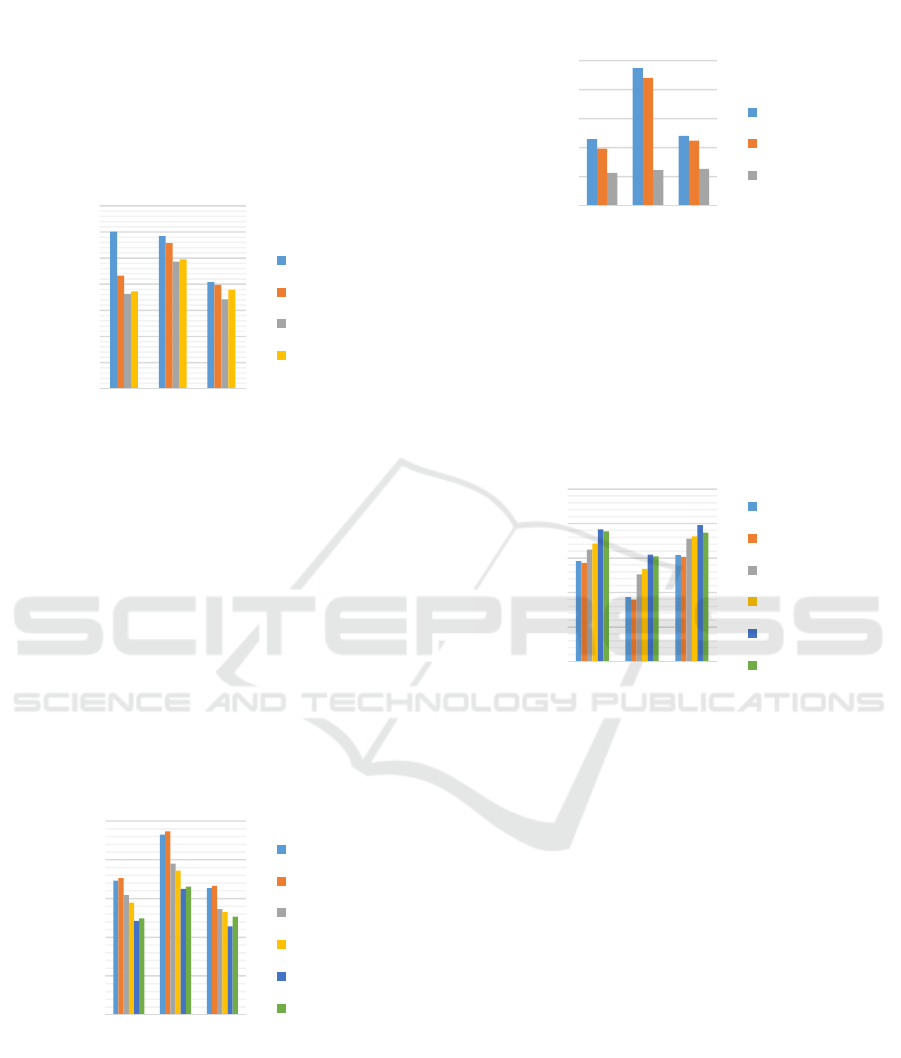
four different DCs, we use the average (12
Cent/KWh) as an electricity price. It was predictable
that PCVM algorithms will outperform other
placement methods. Figure 8b proves the importance
of energy reduction on minimizing the electricity
cost. In general, BF-PCVM and BF-SLA-PCVM
improved the cloud provider electricity cost with an
average of 17% as shown in Figure 8b.
Figure 8b: VM Placement algorithms electricity cost.
Carbon Footprint. Figure 8c studies the
importance of using the CF and PUE factors in
PCVM model in reducing the CO2 footprint under
different number of workload traces. BF-PCVM and
BF-SLA-PCVM compared to BF-LEC (non-carbon
efficient), BF-LCC (non-power efficient), FF-
PCVM and Simple-PCVM (carbon and power
efficient). Based on Figure 8c, BF-PCVM and BF-
SLA-PCVM decrease the CO2 emission with an
average of 16% and 29% compared to other
competing VM placement algorithms. Considering
the algorithms behaviour, we can conclude that the
PUE and CF factors play an important role and lead
to significant reduction in energy and CO2 emission.
Figure 8c: VM placement algorithms’ Carbon Footprint.
SLAH. Figure 8d highlights the importance of BF-
SLA-PCVM in reducing the SLA violation without
ignoring energy saving to minimize the penalties
cost. The experiments show 54% as an average
reduction in SLA violation compared to BF-PCVM
and FF-PCVM algorithms.
Figure 8d: Average percentage of SLAH violation.
Revenue. To calculate the net Revenue per day, the
penalties for missing VM SLA are taken as 10%
refund. Figure 8e illustrates the importance of
PCVM model on increasing the cloud provider net
profit. As Figure 8e shows, BF-PCVM and BF-
SLA-PCVM algorithms outperform other competing
VM placement algorithms.
Figure 8e: VM Placement algorithms net Revenue.
8 CONCLUSION AND FUTURE
WORK
This paper studies the importance of VM placement
decision in geo-distributed DCs. The proposed
PCVM model finds an appropriately suitable host
machine by considering the WAN latency, DC CO2
emission rate, PUE, and energy consumption to
process any user request. The proposed model aims
to assure system QoS, increase environmental
sustainability and improves cloud system’s
operating cost. PCVM-NWP, an intelligent
machine-learning prediction model, is constructed to
improve the performance of the PCVM model by
predicting the weights of the proposed multi-
objective function. Extensive simulations are
conducted and the results show that the proposed
PCVM model can improve cloud provider net profit
by reducing DCs power consumption. Moreover, the
0
500
1000
1500
2000
2500
3000
3500
Day1 Day2 Day3
Electricity Cost ($)
Simple-PCVM
FF-PCVM
BF-PCVM
BF-SLA-PCVM
0
200
400
600
800
1000
Day1 Day2 Day3
Carbon Footprint (Ton)
BF-LCC
BF-LEC
Simple-PCVM
FF-PCVM
BF-PCVM
BF-SLA-PCVM
0
2
4
6
8
10
Day1 Day2 Day3
Average percentage of
SLAH (%)
SLAH
FF-PCVM
BF-PCVM
BF-SLA-PCVM
915
920
925
930
935
940
Day1 Day2 Day3
Revenue ($)
BF-LCC
BF-LEC
Simple-PCVM
FF-PCVM
BF-PCVM
BF-SLA-PCVM
CLOSER 2018 - 8th International Conference on Cloud Computing and Services Science
122

experimental results prove the importance of
considering the communication cost as a parameter
when CSP broker takes the VM placement decision.
As future directions, our aim is to extend the PCVM
model to handle the cost of moving data inside the
modern high-performance network DCs that cause
the main source of power consumption.
REFERENCES
Ahvar, E., Ahvar, S., Crespi, N., Garcia-Alfaro, J. and
Mann, Z. A., 2015, September. NACER: a Network-
Aware Cost-Efficient Resource allocation method for
processing-intensive tasks in distributed clouds.
In Network Computing and Applications (NCA), 2015
IEEE 14th International Symposium on (pp. 90-97).
IEEE
Al-Dulaimy, A., Itani, W., Zekri, A. and Zantout, R.,
2016. Power management in virtualized data centers:
state of the art. Journal of Cloud Computing, 5(1), p.6.
AWS Global Infrastructure. 2017. Available at:
https://aws.amazon.com/about-aws/global-
infrastructure/.[Accessed on January 2017]
Bauer, E. and Adams, R., 2012. Reliability and
availability of cloud computing. John Wiley & Sons
Calheiros, R.N., Ranjan, R., Beloglazov, A., De Rose,
C.A. and Buyya, R., 2011. CloudSim: a toolkit for
modeling and simulation of cloud computing
environments and evaluation of resource provisioning
algorithms. Software: Practice and experience, 41(1),
pp.23-50
Chen, K.Y., Xu, Y., Xi, K. and Chao, H.J., 2013, June.
Intelligent virtual machine placement for cost
efficiency in geo-distributed cloud systems. In
Communications (ICC), 2013 IEEE International
Conference on (pp. 3498-3503). IEEE
eia, US Energy Information Administration. 2017.
Available at: http://www.eia.gov/. [Accessed on
March 2017]
Fan, Y., Ding, H., Wang, L. and Yuan, X., 2016. Green
latency-aware data placement in data
centers. Computer Networks, 110, pp.46-57
Google Data Centers. Google Inc. 2017. Available at:
https://www.google.com/about/datacenters/efficiency/i
nternal/ . [Accessed on March 2017]
Google Inc. Available at: https://www.google.com/
about/datacenters/inside/locations/index.html.
[Accessed on January 2017]
Hall, M., Frank, E., Holmes, G., Pfahringer, B.,
Reutemann, P. and Witten, I.H., 2009. The WEKA
data mining software: an update. ACM SIGKDD
explorations newsletter, 11(1), pp.10-18
Jonardi, E., Oxley, M.A., Pasricha, S., Maciejewski, A. A.
and Siegel, H.J., 2015, December. Energy cost
optimization for geographically distributed
heterogeneous data centers. In Green Computing
Conference and Sustainable Computing Conference
(IGSC), 2015 Sixth International (pp. 1-6). IEEE
Khosravi, A., Garg, S.K. and Buyya, R., 2013, August.
Energy and carbon-efficient placement of virtual
machines in distributed cloud data centers. In
European Conference on Parallel Processing
(pp. 317-328). Springer, Berlin, Heidelberg
Luckow, P., et al. "Spring 2016 National Carbon Dioxide
Price Forecast." (2016).
Malekimajd, M., Movaghar, A. and Hosseinimotlagh, S.,
2015. Minimizing latency in geo-distributed clouds.
The Journal of Supercomputing, 71(12), pp.4423-4445
Pereira, F., Mitchell, T. and Botvinick, M., 2009. Machine
learning classifiers and fMRI: a tutorial overview.
Neuroimage, 45(1), pp.S199-S209
Planet lab traces, Available at: https://www.planet-lab.org,
[Accessed on January 2017].
Rawas, S., Itani, W., Zaart, A. and Zekri, A., 2015,
October. Towards greener services in cloud
computing: Research and future directives. In
Applied Research in Computer Science and
Engineering (ICAR), 2015 International Conference
on (pp. 1-8). IEEE.
Signiant organization. 2017. Available at:
http://www.signiant.com/products/flight/pricing/
Standard Performance Evaluation Corporation. 2017.
Available at: http://www.spec.org, [Accessed on
January 2017]
Sverdlik, Y., 2014. Survey: Industry average data center
pue stays nearly flat over four years. Data Center
Knowledge, 2(06)
Thang, K., 2015. Estimated social cost of climate change
not accurate, Stanford scientists say. Retrieved
June, 5, p.2016
Wan Latency Estimator. Available at: http://wintelguy.
com/wanlat.html. [Accessed on February 2017]
Weinberger, K.Q. and Saul, L.K., 2009. Distance metric
learning for large margin nearest neighbor
classification. Journal of Machine Learning Research,
10(Feb), pp.207-244
Zhou, Z., Liu, F., Xu, Y., Zou, R., Xu, H., Lui, J.C. and
Jin, H., 2013, August. Carbon-aware load balancing
for geo-distributed cloud services. In Modeling,
Analysis & Simulation of Computer and
Telecommunication Systems (MASCOTS), 2013 IEEE
21st International Symposium on (pp. 232-241). IEEE
Power and Cost-aware Virtual Machine Placement in Geo-distributed Data Centers
123
