
Land-use Classification for High-resolution Remote Sensing Image
using Collaborative Representation with a Locally Adaptive
Dictionary
Mingxue Zheng
1,2
and Huayi Wu
1
1
Key Laboratory of Information Engineering in Surveying, Mapping, and Remote Sensing, Wuhan University, Wuhan, China
2
Faculty of Architecture and the Built Environment, Delft University of Technology, Delft, The Netherlands
Keywords: Classification, Locally Adaptive Dictionary, Collaborative Representation, High-Resolution Remote Sensing
Image.
Abstract: Sparse representation is widely applied in the field of remote sensing image classification, but sparsity-based
methods are time-consuming. Unlike sparse representation, collaborative representation could improve the
efficiency, accuracy, and precision of image classification algorithms. Thus, we propose a high-resolution
remote sensing image classification method using collaborative representation with a locally adaptive
dictionary. The proposed method includes two steps. First, we use a similarity measurement technique to
separately pick out the most similar images for each test image from the total training image samples. In this
step, a one-step sub-dictionary is constructed for every test image. Second, we extract the most frequent
elements from all one-step sub-dictionaries of a given class. In the step, a unique two-step sub-dictionary, that
is, a locally adaptive dictionary is acquired for every class. The test image samples are individually
represented over the locally adaptive dictionaries of all classes. Extensive experiments (OA (%) =83.33,
Kappa (%) =81.35) show that our proposed method yields competitive classification results with greater
efficiency than other compared methods.
1 INTRODUCTION
Recently, high-resolution remote sensing images
(HRIs) have been frequently occurred in many
practical applications, such as in Cascaded
classification (Guo et al., 2013), urban area
management (Huang et al., 2014), and residential area
extraction (Zhang et al., 2015). Especially, HRIs play
an increasingly important role in land-use
classification (Chen and Tian, 2015; Hu et al., 2015;
Zhao et al., 2014). Natural images, are generally
sparse, and therefore can be sparsely represented and
classified (Olshausen and Field, 1997). Sparse
Representation based Classification (SRC) (Wright et
al., 2009) was a sparse linear combination of
representation bases, i.e. a dictionary of atoms, and
had been successfully applied in the field of image
classification (Yang et al., 2009). But sparsity based
methods were time-consuming. In contrast to sparsity
based classification algorithms, Collaborative
Representation based Classification (CRC) (Zhang et
al., 2011) yielded a very competitive level of
accuracy with a significantly lower complexity. In
(Zhang et al., 2012), Zhang et.al pointed out that it
was Collaborative Representation (CR) that can
represent test image collaboratively with training
image samples from all classes, as image samples
between different classes often share certain
similarity. In (Li and Du, 2014; Li et al., 2014), Li
et.al proposed two methods, Nearest Regularized
Subspace (NRS) and Joint Within-Class
Collaborative Representation (JCR), for
hyperspectral remote sensing images classification.
These methods also could probably be extended to
classify for HRIs. The essence of a NRS classifier
was a
penalty framed as a distance weighted
Tikhonov regularization. This distance weighted
measurement enforced a weight vector structure.
Unlike the sparse representation based approach, the
weights can be simply estimated through a
closed-form solution, resulting in much lower
computational cost, but the method ignored the
spatial information at neighboring locations. To
overcome this disadvantage of NRS, JCR was
88
Zheng, M. and Wu, H.
Land-use Classification for High-resolution Remote Sensing Image using Collaborative Representation with a Locally Adaptive Dictionary.
DOI: 10.5220/0006705300880095
In Proceedings of the 4th International Conference on Geographical Information Systems Theory, Applications and Management (GISTAM 2018), pages 88-95
ISBN: 978-989-758-294-3
Copyright
c
2019 by SCITEPRESS – Science and Technology Publications, Lda. All rights reserved

proposed. Both methods enhanced classification
precision, but also created a serious problem as
irrelevant estimated coefficients generated during
processing were scattered over all classes, instead of
concentrated in a particular one, therefore adding
uncertainty to the final classification results.
Additionally, these methods just considered the first
“joint” of the original training samples, and forewent
a second deep selection from them, which could be
the basis of a more complete and non-redundant
dictionary for HRI classification.
In this paper, we focus on the CR working
mechanism, and propose a high-resolution remote
sensing image classification method using CR with a
locally adaptive dictionary (LAD-CRC).The
LAD-CRC method makes up of two stages. First, we
use a similarity measure to separately pick out the
most similar images for each test image from the total
training sample images, constructing a one-step
sub-dictionary for each test image. Second, each test
image will share certain similarities with some of the
training images, the one-step sub-dictionaries for
these test images therefore highly correlate. Based on
this correlation, we extract the most frequent
elements from all one-step sub-dictionaries of total
test images in a given class, and construct a two-step
sub-dictionary for the given class. The total of the
most frequent elements, that is, two-step
sub-dictionary, means the locally adaptive dictionary
of the given class. A test image therefore share a
unique two-step sub-dictionary with the other test
images in the same class. We also call two-step
sub-dictionary per class as a locally adaptive
dictionary. Test images are individually represented
by the locally adaptive dictionaries of all classes.
Extensive experiments show that our proposed
method not only increases classification precision,
but also decreases computing time.
The remaining parts of this paper are organized as
follows. Section 2 discusses basic CR theory. Section
3 details the proposed algorithm. Section 4 describes
experimental results and analysis of the proposed
algorithm. Conclusions are drawn in section 5.
2 BASIC THEORY
In this section, we will introduce the general CR
model with corresponding regularizations, for
reconstructing a test image.
2.1 Collaborative Representation (CR)
Suppose that we have C classes of training samples,
and all training image samples are denoted by.
Denote by
the
training image
sample of the
class, and denote by
the training image samples of the
class,
then let
,
.When giving a test sample
from
the class i, we represent it as
(1)
where
and
is the coefficient
associated with the class i, is a small threshold. A
general CR model can be represented as
(2)
where p and q equal to one or two. Different settings
of p and q lead to different instantiations.
2.2 Reconstruction and Classification of
HRIs via CR
The working mechanism of CR is that some
high-resolution remote sensing images from other
classes can be helpful to represent the test image
when training images belonging to different classes
share certain similarities. The USA land-use dataset
in our experiment is a small sample size problem, and
is under-complete in general. If we use
to
represent the test image y, the representation error
will be very large, even when y belongs to the class i.
One obvious solution to solve the problem is to use
much more training samples to represent the test
image y. For HRIs, we experimentally set p as two, q
as one, and the Lagrange dual form of this case can be
shown as
(3)
where the parameter λ is a tradeoff between the data
fidelity term and the coefficient prior. We compute
the residuals
, then
identify the class of the test image y via
.
3 THE PROPOSED METHOD
In this section, we will detail how to extract
sub-dictionaries at each step, finally obtain a locally
adaptive dictionary. We will present the complete
algorithm process in the proposed method for HRI
classification.
Land-use Classification for High-resolution Remote Sensing Image using Collaborative Representation with a Locally Adaptive Dictionary
89

3.1 Feature Extraction
The set of features adopted in land-use classification
(Mekhalfi et al., 2015) consisted of three types as
follows: Histogram of Oriented Gradients (HOG)
(Dalal and Triggs, 2005), Cooccurrence of Adjacent
Local Binary Patterns (CoALBP) (Nosaka et al.,
2011) and Gradient Local AutoCorrelations (GLACs)
(Kobayashi and Otsu, 2008). The results showed the
CoALBP produced the most accurate land use
classification results. In our work, CoALBP features
are utilized to construct the sub-dictionaries from the
land-use dataset. In the representation format with
CoALBP features, a high resolution remote sensing
image is represented by a column vector.
3.2 One-step Sub-dictionary
Suppose we have C classes of test samples, all test
samples are denoted by, the test samples of
class are denoted by
Denote by
the
test sample of the
class. As mentioned in
2.1, denote by
the training samples of
the
class, then let
. Because of similarity among image samples,
we just need to choose the most similar training
samples for every test image, instead of complete
training image samples. Here, we use similarity
measurement principle to select out the most similar S
training images in every
to construct an one-step
sub-dictionary of
, denoted by
(4)
is the sample set that includes the most
similar S training samples of the
class with test
image
,where
And
are respectively subsets
of
is the number of elements
in subset
. The mathematical function of
similarity measurement principle is as follow
(5)
where
are n vectors. The smaller the d
value, the more similar x and y.
3.3 Two-step Sub-dictionary
From the section 3.2, the one-step sub-dictionary of
all test samples of the
class, denoted by
]
(6)
where
(7)
are all selected training samples of the
class. The
two-step sub-dictionary, that is, the S samples that
frequently occur in
, denoted by
(8)
All new selected training samples of the
class is
denoted by
the number is
,
and
. The locally adaptive dictionary
of
class is
.
3.4 The Flow of the Proposed Method
for HRIs Classification
To summarize the proposed method, we show the
following steps.
1) Given a test image
of the
class, a
similarity measurement principle is used to
construct an one-step sub-dictionary of
from total training images of all classes, denoted
by
(9)
After doing same process for other test images
of the
class, the one-step sub-dictionary of the
class is
;
2) A two-step sub-dictionary of the
class, that
is, the first S columns those occur repeatedly
in
is construct, denoted by
(10)
is also called the locally adaptive dictionary
of the
class;
3) From the foregoing, we can obtain the proposed
method as
} (11)
where
refers to the local coefficient matrix
corresponding to the locally adaptive dictionary
, and
;
GISTAM 2018 - 4th International Conference on Geographical Information Systems Theory, Applications and Management
90
4) After traversing all the classes, we get a global
coefficient matrix. The label of the test HRI
is determined by the following classification
rule
(12)
where
is a subpart of associated with the
class i and
denotes the portion of the
recovered collaborative coefficients
for the
class.
5) In sequence, we can get a 2-D matrix which
records the labels of the HRIs in the last.
Additionally, the specific scheme for the global
coefficient matrix construction is shown as follows.
Global coefficient matrix
construction
Input: (1) The local coefficient matrix
;
(2) Indicator set I with N elements, and
, or
1, for , in which “1” means that the
corresponding dictionary atom is active and “0”
means inactive.
Initialization: Set the initial global coefficient matrix
as a zero matrix, and an indicator v
=1.
For i = 1 to N
if
;
=
;
v ++ ;
End if
End For
Output: The global coefficient matrix
4 RESULT AND ANALYSIS
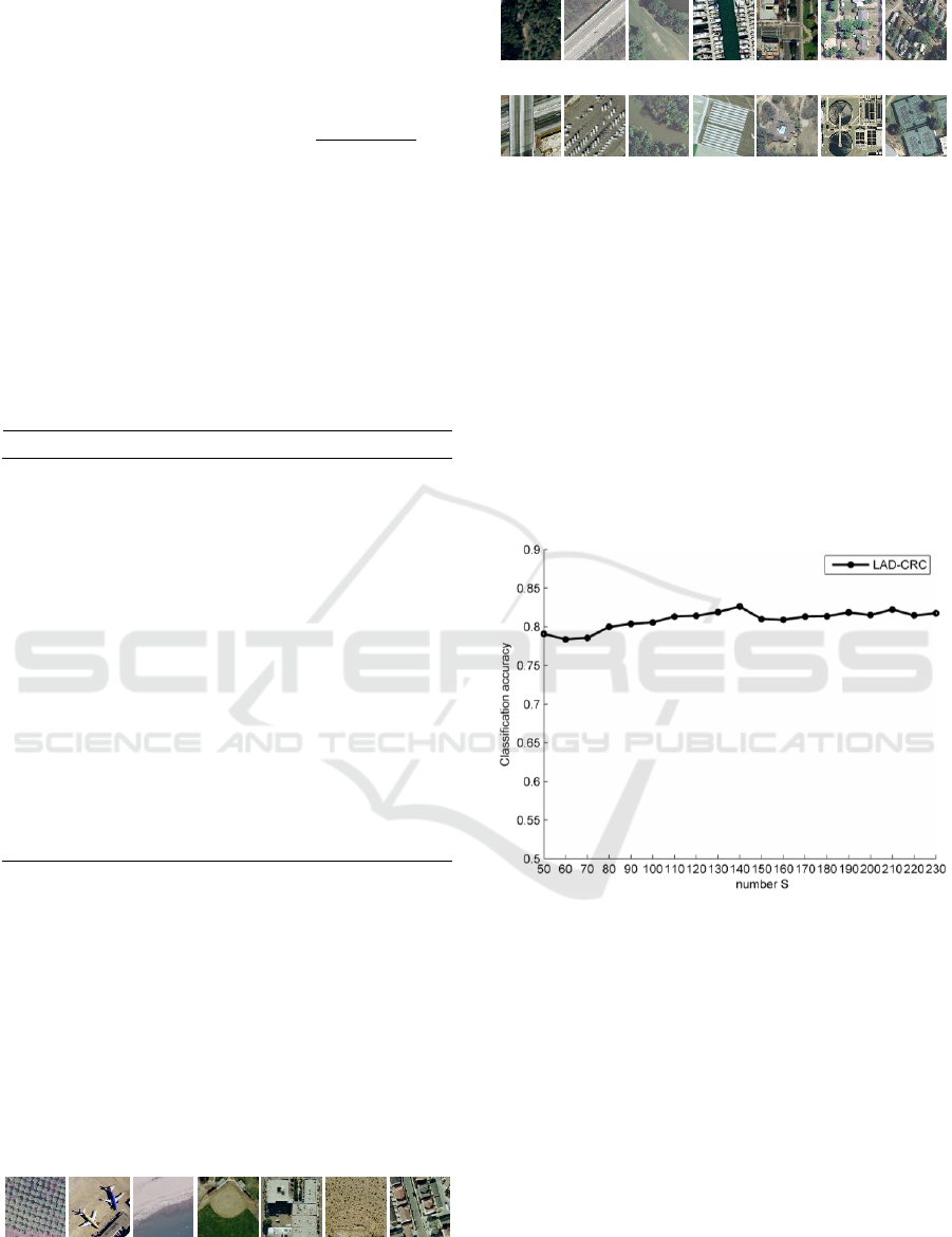
The USA land-use dataset (Yang and Newsam, 2010)
is widely used for evaluating land-use classification
algorithms. It includes 21 classes, each class has 100
images. 80 images are selected out as training
samples per class, other 20 images per class are test
samples. Then, the total number of training samples is
1680. Image samples of each land-use class are
shown in Figure 1.
1
2
3
4
5
6
7
8
9
10
11
12
13
14
15
16
17
18
19
20
21
Figure 1: Example images of USA land-use dataset.
(1 agriculture; 2 airplane; 3 baseball diamond; 4 beach;
5 buildings; 6 chaparral; 7 dense residential; 8 forest; 9
freeway; 10 golf course; 11 harbor; 12 intersection; 13
medium residential; 14 mobile phone park; 15
overpass; 16 parking lot; 17 river; 18 runway; 19
sparse residential; 20 storage tanks; 21 tennis court).
4.1 Parameter Setting
The selection of sample number S in two steps is
critical in LAD-CRC. Experimentally, we set the S
value equal to 210.
Figure 2: The S value of locally adaptive dictionary per
class.
In Figure 2, it shows the relationship between the
number S of locally adaptive dictionary per class and
the classification accuracy. The range of the number
S in LAD-CRC is [50, 230], the step length is 10.
There are two convex points with S equal to 140 and
210. The accuracy values on these two points are
almost the same. But the accuracy tread is more stable
around 210. In addition, 140 is not a suitable value as
we compress the 1x1680 estimated coefficient vector
to a 1x210 coefficient vector to show the rough
distribution of estimated coefficients for all methods.
It is more clear and concise to show the distribution of
coefficients with the 1x210 vector. The regularized
parameter λ is 0.1 in NRS and JCR, 0.001 in SRC and
Land-use Classification for High-resolution Remote Sensing Image using Collaborative Representation with a Locally Adaptive Dictionary
91
CRC experimentally. Other parameters are the same
in all five methods.
4.2 Result Comparison with Other
Methods
Using the USA land-use dataset, we conduct many
experiments to compare with results of SRC (Wright
et al., 2009), CRC (Wright et al., 2009), NRS (Li et
al., 2014), and JCR (Li and Du, 2014), algorithms.
Classification accuracy is averaged over five
cross-validation evaluations. To facilitate a fair
comparison between our proposed algorithm and
other approaches, a fivefold cross-validation is
performed in which the dataset is randomly
partitioned into five equal subsets. After portioning,
each land-use class contains a subset of 20 images.
Four of these subsets are used for training, while the
remaining subset is used for testing. The results
include average accuracy (OA) of all classes and
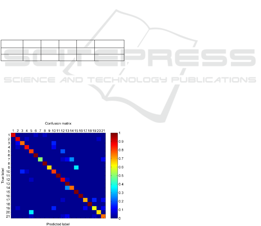
Kappa coefficients are showed in Table 1.
Table 1: Classification results for USA land-use dataset
with the proposed LAD-CRC.
SRC
CRC
NRS
JCR
LAD-CRC
OA (%)
66.95
55.81
71.71
71.10
83.33
Kappa (%)
66.50
52.25
69.75
70.30
81.35
In Table 1, the compared results show that the
locally adaptive dictionary in proposed method can
greatly replace the whole dictionary (e.g., the whole
training image samples), and improves classification
accuracy (OA=83.33; Kappa=81.35). The idea of
extracting two sub-dictionaries refines the
information of total training sample information into
a locally adaptive dictionary.
Figure 3: Confusion matrix for the land-use data set using
the proposed method.
The average classification performances of the
individual classes using our proposed method set with
the optimal parameters are visually shown in the
confusion matrix (Figure 3).The average accuracies
occur along a diagonal shown in red to yellow cells in
the figure, mostly focusing on 82.620.71%.
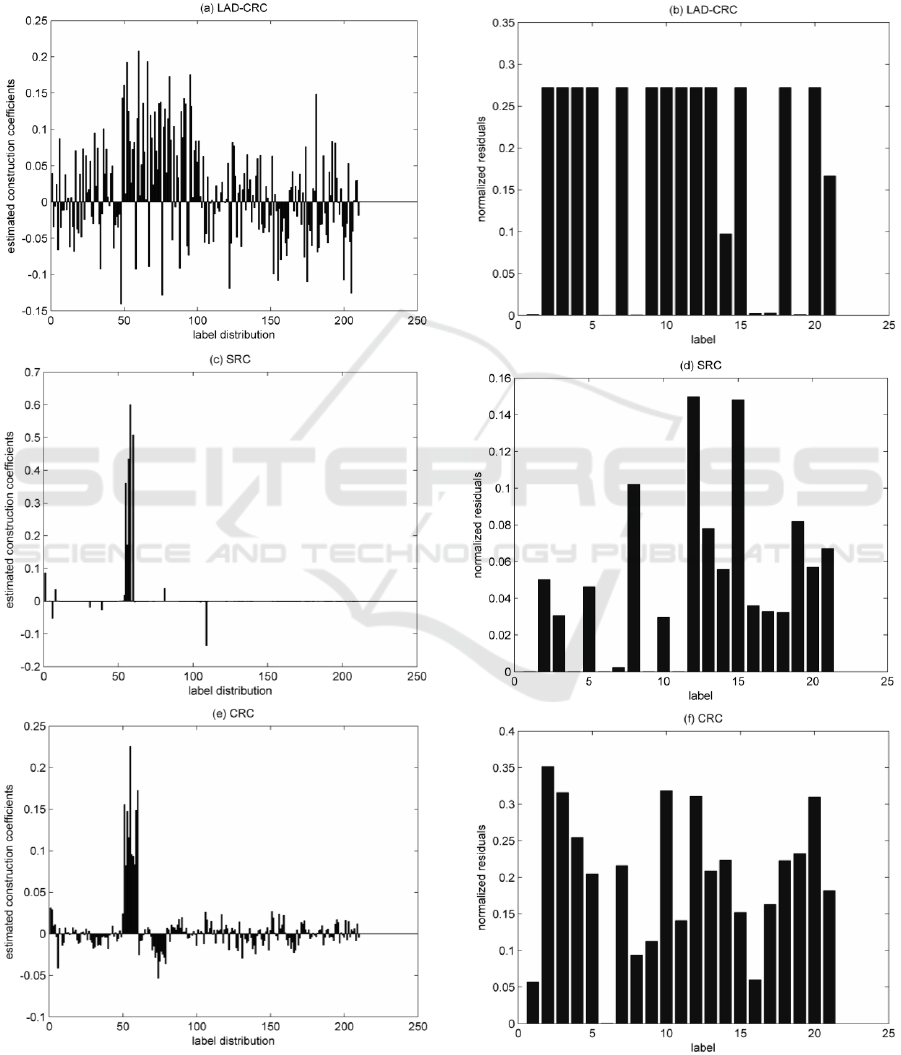
Without loss of generality, in this paper, we
randomly choose the fifteenth test image sample of
the class 6 in fifth cross-validation dataset, to
demonstrate classification performance of the
proposed method. In Figure 4, Figure 4(a)-(j) show
estimated construction coefficients and normalized
residuals for all five methods. Figure 4(a), 4(c), 4(e),
4(g), and 4(i) show estimated construction
coefficients, and the variable on x axis is the
distribution of training samples for all 21 classes
(e.g., label distribution), the range of training samples
of the class 6 is [20, 101] in Figure 4(a), [51, 60] in
Figure 4(c), 4(e), 4(g), and 4(i). The value on y axis is
corresponding estimated construction coefficients of
different classes. Figure 4(b), 4(d), 4(f), 4(h), and 4(j)
show normalized residuals of different classes. It can
be observed that all the approaches can identify the
test sample image properly by the rule of the least
error, but the coefficient values for different
algorithms are largely different. From Figure 4 (a)
and 4(b), estimated construction coefficients mostly
locate on class 6 (from 20 to101 on the x axis), 8
(from 102 to 178 on the x axis), 17(from 182 to190 on
the x axis) and 19(from 191 to 209 on the x axis), but
there has the least normalized residuals in class 6,
which means proposed method mainly unitizes
training sample images in class 6 to construct the test
sample image. From Figure 4(c) and 4(d) in SRC, the
normalized residuals in class 1,4,6,9 and 11 all are
little, and estimated construction coefficients almost
focus on class 6 (from 51 to 60 on the x axis), it means
that the test sample image is reconstructed by training
sample images in class 6. Similarly, from Figure 4(e)
and 4(f) in CRC, estimated construction coefficients
mainly locate in class 6 (from 51 to 60 on the x axis),
and normalized residual in class 6 obviously is the
smallest. In NRS and JCR, from Figure 4(g) and 4(i),
the distributions of estimated construction
coefficients are irregular. But from Figure 4(h) and
4(j), the normalized residual on class 6 still is the
smallest.
Compared Figure 4(a) with 4(c), 4(e), there are
many disturbances (estimated construction
coefficients in class 8, 17 and 19). There are two
reasons for these noises: (1) Due to the selection of
sub-dictionaries at two steps, 210 selected training
sample images are very similar to the test sample
image of the class 6; (2)Even though 210 selected
GISTAM 2018 - 4th International Conference on Geographical Information Systems Theory, Applications and Management
92
training image samples mostly belong to the class 6,
training sample images probably share certain
similarity among some classes. Then, there should be
some training samples of other classes in the 210
selected training samples. We call these classes
“similar class”, such as class 8, 17, and 19. The
situations in such two reasons result that a part of
estimated construction coefficients of the test image
are scattered in “similar classes”. The distribution of
normalized residuals in Figure 4(b) perfectly match
the fact “similar class” causes. The coefficient
disturbances of LAD-CRC just locate on “similar
Figure 4: estimated construction coefficients and normalized residuals among all method.
Land-use Classification for High-resolution Remote Sensing Image using Collaborative Representation with a Locally Adaptive Dictionary
93
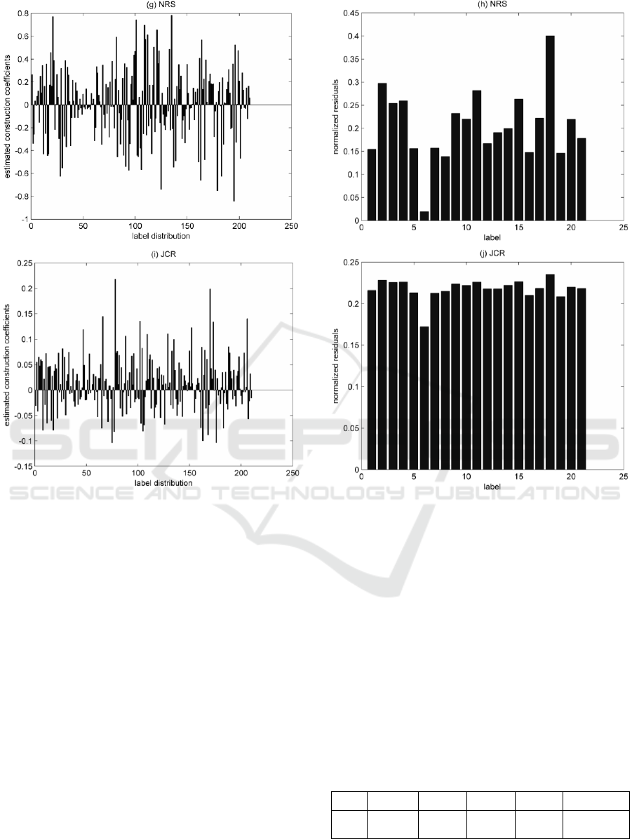
Figure 4: estimated construction coefficients and normalized residuals among all method (cont.).
class”. In addition, the estimated construction
coefficients of CRC locate on all classes. Estimated
construction coefficients in other classes make the
very serious impact on computing residuals, which
results that CRC achieves the worst classification
result.
Compared Figure 4(a) with Figure 4(g), 4(i), these
irregular reconstruction coefficient distribution in
Figure 4(g) and 4(i) perfectly prove the validity of
proposed method by refining the information of total
training sample information into a locally adaptive
dictionary.
To conclude, considering that all methods can
identify the test image sample properly, the proposed
method can select the most valuable training image
samples. With the construction of a locally adaptive
dictionary, we receive the best classification
accuracy.
However, it is easy to find that the results of four
compared algorithms are approximately 10% lower
than these they acquired in other datasets. We could
give the probable reason. Generally, SIFT is the most
common feature descriptor for HRI classification. In
the paper, we choose CoALBP features to collect
HRIs information. LBP is a descriptor for rotation
invariant texture classification. CoALBP is the
extension of LBP to extract finer local details. The
reason we choose CoALBP instead of SIFT is that the
feature exploitation with the latter will take much
more computation time than the former takes.
Fortunately, the phenomenon that results are lower
than these methods acquired in other datasets exists in
all four compared algorithms without a special case.
So the comparison results in Table 1 still can testify
the performance of the proposed method, even under
the impact of CoALBP features.
Table 2: Speed for USA land-use dataset.
SRC
CRC
NRS
JCR
LAD-CRC
Time
(s)
5018.957
7.4216
26.8122
35.3689
2215.7087
In Table 2, the computation time each method
consumes is showed. The computation time including
GISTAM 2018 - 4th International Conference on Geographical Information Systems Theory, Applications and Management
94

training and test processes the proposed method takes
is less than SRC takes, but more than CRC, NRS and
JCR take. In Table 2, the more accurate a method is,
the more computation time is generally required. This
demonstrates that accuracy comes at the cost of
increasing computational efforts. It is time
consuming to separately find out the most similar
training images for each test image and the most
frequent training images for every class with two
sub-dictionaries. The process occupies most of the
running time of the proposed method.
5 CONCLUSION
In this paper, experimental results clearly show that
the proposed method obtains the best classification
performance. It means the idea of training
dictionaries at two steps is promising, and encourages
me further to explore the direction. From Figure 4(a),
there still are many disturbances (for example,
estimated construction coefficients in class 8, 17 and
19). Effective methods for extracting discriminative
information of different classes should be explored to
decrease and even eliminate these disturbances.
Besides, time consuming on sub-dictionaries is also a
problem. To find out a way to reduce computing time
is necessary. Parallel computing can be thought as an
ideal direction in the future work.
REFERENCES
Chen, S., Tian, Y., 2015. Pyramid of spatial relatons for
scene-level land use classification. IEEE Transactions
on Geoscience and Remote Sensing 53, 1947-1957.
Dalal, N., Triggs, B., 2005. Histograms of oriented
gradients for human detection, Computer Vision and
Pattern Recognition, 2005. CVPR 2005. IEEE
Computer Society Conference on. IEEE, pp. 886-893.
Guo, J., Zhou, H., Zhu, C., 2013. Cascaded classification of
high resolution remote sensing images using multiple
contexts. Information Sciences 221, 84-97.
Hu, F., Xia, G.-S., Hu, J., Zhang, L., 2015. Transferring
deep convolutional neural networks for the scene
classification of high-resolution remote sensing
imagery. Remote Sensing 7, 14680-14707.
Huang, X., Lu, Q., Zhang, L., 2014. A multi-index learning
approach for classification of high-resolution remotely
sensed images over urban areas. ISPRS Journal of
Photogrammetry and Remote Sensing 90, 36-48.
Kobayashi, T., Otsu, N., 2008. Image feature extraction
using gradient local auto-correlations, European
conference on computer vision. Springer, pp. 346-358.
Li, W., Du, Q., 2014. Joint within-class collaborative
representation for hyperspectral image classification.
IEEE Journal of Selected Topics in Applied Earth
Observations and Remote Sensing 7, 2200-2208.
Li, W., Tramel, E.W., Prasad, S., Fowler, J.E., 2014.
Nearest regularized subspace for hyperspectral
classification. IEEE Transactions on Geoscience and
Remote Sensing 52, 477-489.
Mekhalfi, M.L., Melgani, F., Bazi, Y., Alajlan, N., 2015.
Land-use classification with compressive sensing
multifeature fusion. IEEE Geoscience and Remote
Sensing Letters 12, 2155-2159.
Nosaka, R., Ohkawa, Y., Fukui, K., 2011. Feature
extraction based on co-occurrence of adjacent local
binary patterns, Pacific-Rim Symposium on Image and
Video Technology. Springer, pp. 82-91.
Olshausen, B.A., Field, D.J., 1997. Sparse coding with an
overcomplete basis set: A strategy employed by V1?
Vision research 37, 3311-3325.
Wright, J., Yang, A.Y., Ganesh, A., Sastry, S.S., Ma, Y.,
2009. Robust face recognition via sparse
representation. IEEE transactions on pattern analysis
and machine intelligence 31, 210-227.
Yang, J., Yu, K., Gong, Y., Huang, T., 2009. Linear spatial
pyramid matching using sparse coding for image
classification, Computer Vision and Pattern
Recognition, 2009. CVPR 2009. IEEE Conference on.
IEEE, pp. 1794-1801.
Yang, Y., Newsam, S., 2010. Bag-of-visual-words and
spatial extensions for land-use classification,
Proceedings of the 18th SIGSPATIAL international
conference on advances in geographic information
systems. ACM, pp. 270-279.
Zhang, L., Yang, M., Feng, X., 2011. Sparse representation
or collaborative representation: Which helps face
recognition?, Computer vision (ICCV), 2011 IEEE
international conference on. IEEE, pp. 471-478.
Zhang, L., Yang, M., Feng, X., Ma, Y., Zhang, D., 2012.
Collaborative representation based classification for
face recognition. arXiv preprint arXiv:1204.2358.
Zhang, L., Zhang, J., Wang, S., Chen, J., 2015. Residential
area extraction based on saliency analysis for high
spatial resolution remote sensing images. Journal of
Visual Communication and Image Representation 33,
273-285.
Zhao, L.-J., Tang, P., Huo, L.-Z., 2014. Land-use scene
classification using a concentric circle-structured
multiscale bag-of-visual-words model. IEEE Journal of
Selected Topics in Applied Earth Observations and
Remote Sensing 7, 4620-4631.
Land-use Classification for High-resolution Remote Sensing Image using Collaborative Representation with a Locally Adaptive Dictionary
95
