
Managing Graph Modeling Alternatives for Link Prediction
Silas P. Lima Filho, Maria Claudia Cavalcanti and Claudia Marcela Justel
Military Institute of Engineering, Praca General Tiburcio 80, Urca, Rio de Janeiro, Brazil
Keywords:
Modelling Formalism, Link Prediction, Heuristics.
Abstract:
The importance of bringing the relational data to other models and technologies has been widely debated, as
for example their representation as graphs. This model allows to perform topological analysis such as social
analysis, link predictions or recommendations. There are already initiatives to map from a relational database
to graph representation. However, they do not take into account the different ways to generate such graphs
from data stored in relational databases, specially when the goal is to perform topological analysis. This work
discusses how graph modeling alternatives from data stored in relational datasets may lead to useful results.
However, this is not an easy task. The main contribution of this paper is towards managing such alternatives,
taking into account that the graph model choice and the topological analysis to be used, depend on the links the
user intends to predict. Experiments are reported and show interesting results, including modeling heuristics
to guide the user on the graph model choice.
1 INTRODUCTION
One of the reasons to convert data stored in relational
databases into graph representation models is to sup-
port “decision-making”. For decades the graph model
has been widely explored in topological analysis, and
there are plenty of algorithms and applications on the
literature. Usually, these algorithms have been app-
lied in the context of social network, recommendation
systems, link prediction and many others.
In this direction, some alternatives to map relati-
onal data into graphs, more specifically RDF graphs,
came up, such as D2R (Bizer, 2003). However, such
initiatives focus on syntax mapping, and do not ad-
dress graph modeling issues. On the other hand, there
are works (Virgilio et al., 2014b) (Wardani and Kng,
2014) (Bordoloi and Kalita, 2013) that focus on graph
modeling, but embrace a specific modeling strategy
and do not take into account modeling strategy alter-
natives, nor the intended topological analysis.
The goal of this paper is to demonstrate that the
use of alternative modelings can provide richer infe-
rences, such as to recommend different pairs of rela-
ted objects, or to predict different types of links. The
key idea consists on assisting the user on the task of
graph modeling, based on the analysis of a conceptual
schema, derived from a relational schema of a data-
base. The main contribution is the identification of a
set of heuristics, which take into account the intended
topological analysis and guides the user on choosing
the modelings that may be useful. These heuristics
were identified based on the results of some experi-
ments using topological analysis (e.g. link prediction)
over different modeling choices.
This work is organized as follows: Section 2 pre-
sents some basic concepts that are used throughout
the paper. Section 3 describes the related works on
graph database modeling and on mapping the relati-
onal data to graph structures. Section 4 presents the
motivation for deriving heuristics and describes how
the experiments were conducted. Section 5 presents
the experiments, as well as their results, and also pre-
sents the heuristics that emerged based on them. Fi-
nally, the last section concludes the work, pointing to
some future directions.
2 BASIC FOUNDATIONS
This section presents basic concepts about social net-
work analysis, graph modeling and relational data-
base modeling.
2.1 Social Networks Analysis
Social networks have received much attention in the
last years because they allow to model relationships
between actors, like people or other objects. For in-
stance, friendship, influence and collaboration net-
P. Lima Filho, S., Claudia Cavalcanti, M. and Marcela Justel, C.
Managing Graph Modeling Alternatives for Link Prediction.
DOI: 10.5220/0006708700710080
In Proceedings of the 20th International Conference on Enterprise Information Systems (ICEIS 2018), pages 71-80
ISBN: 978-989-758-298-1
Copyright
c
2019 by SCITEPRESS – Science and Technology Publications, Lda. All rights reserved
71

works, biological networks, electric distribution net-
works, pages and web links computer networks, were
presented in several applications (Easley and Klein-
berg, 2010). There are different ways to analyze so-
cial networks. We will focus our work in topological
analysis, that is, we model the network as a graph, and
use algorithms to obtain information about degree of
nodes, paths and distances between nodes.
Because of its nature, the social networks are
highly dynamic, that is, they change fast over the
time, by the adding of new nodes or edges. One of the
questions about the dynamic of the network is, how
does the association between nodes change over the
time? We are interested in predict future association
between nodes, knowing that there is no association in
the current state of the graph. This problem is known
as Link Prediction (Aggarwal, 2011).
Nowell and Kleinberg (Liben-Nowell and Klein-
berg, 2007) have adapted some concepts from graph
theory, computer science and social studies as metrics
to determine future connections to be inserted in the
graph. Three formulas have been used in our experi-
ments, taken from Nowell and Kleinberg article, and
can be classified in two types of metrics: one based
in common neighbors and other based in path assem-
bling. All the considered metrics produce a coeffi-
cient for a pair of nodes x, y non connected by an edge
in the graph. Common neighbors metrics analyze in
different ways the number of common neighbors of
x and y. Path assembling metrics measures in some
sense the paths between a pair of nodes in the graphs.
Jaccard and Adamic/Adar coefficients are classi-
fied as common neighbors metrics, meanwhile Katz
coefficient as path assembling metric. Jaccard coef-
ficient is stated by: score(x;y) =
|Γ(x)∩Γ(y)|
|Γ(x)∪Γ(y)|
. The
Adamic/Adar coefficient is defined by: score(x;y) =
∑
z∈Γ(x)∩Γ(y)
1
log(|Γ(z)|)
. And Katz coefficient is:
score(x, y) =
∑
∞
l=1
β
l
|paths
l
x,y
|, where paths
l
x,y
is the
set with all the paths with length l between nodes x, y,
and β is an arbitrary value. In our experiments, we
defined β =
1
λ
1
, and λ
1
is the greatest eigenvalue of
the adjacency matrix of the graph.
2.2 Relational and Graph Modeling
Heuser (Heuser, 2009) states that a data model must
be expressive enough to create database schemas. In
other words, it must be sufficiently expressive for mo-
deling reality into schemas. Designing a database
schema is a task which usually goes through two steps
with different level of abstraction: conceptual and lo-
gical modeling. These two steps are needed due to
the complexity of the reality that the designer intends
to model. The main idea is to conduct the modeler
from the reality level into some logical data struc-
ture that may represent real objects. The ER model
(Chen, 1976) is commonly used to design conceptual
schemas, where objects and relationships of the real
world are represented as entities (classes of objects)
and their relationship types (see Figure 1). In the
second step, these entities and relationships are then
mapped into a logical schema. The Relational Model
(Codd, 1970) is largely used to create logical sche-
mas, where tables are defined as the structures that
will actually store the data. For instance, if the dom-
ain involves actors and movies, these can be modeled
as entities 1 and 2, and the participation that an actor
can have in a movie can be modeled as a relationship
between those two entities.
Figure 1: Suggested model for an general situation.
Different from database modeling, that aims at
the storage and management of data, graph modeling
aims at data analysis, such as social network analy-
sis or, in particular link prediction. The need to ad-
dress both goals has led to the rise of graph oriented
DBMS (GDBMS). These systems use a graph struc-
ture to store data. Neo4J
1
is one of the most used
GDBMS.
Rodriguez (Rodriguez and Neubauer, 2010)
points to several different graph structures. For ex-
ample, some graph structures are able to represent
different features for each vertex or edge, such as la-
bels, attributes, weight, etc. In his article, he presents
a hierarchic classification, where graph structures are
organized according to their expressivity (number of
features allowed). The structure known as property
graph, is the most commonly used by graph manipu-
lation tools (e.g. Neo4J), due to its expressiveness.
Graphs may be modeled based on data items that
come from databases. In order to map data items from
a relational database to a graph structure, it is neces-
sary to count on both conceptual and logical sche-
mas. The modeler can use them to identify which data
items will be represented as vertices, and which refe-
rences can become edges in the graph database. Ho-
wever, this is not an easy task, specially when there is
a variety of analysis that can be performed.
The following section presents some initiatives in
this direction. However, to the best of our knowledge,
there are no methods or guidelines to assist the graph
modeler in doing such task, taking into account the
analysis to be performed.
1
http://neo4j.com/developer/example-data/
ICEIS 2018 - 20th International Conference on Enterprise Information Systems
72

3 RELATED WORK
Some works have already approached the task of
graph modeling based on data from the relational mo-
del databases. One of them (Virgilio et al., 2014b)
focus on graph modeling aiming at the improvement
of query performance on the graph database. Diffe-
rently, another work (Wardani and Kng, 2014) focus
on avoiding semantic losses while modeling, whereas
in (Bordoloi and Kalita, 2013) the focus is on avoi-
ding data redundancy.
The main idea of Wardani and K
¨
ung’s work (War-
dani and Kng, 2014) is to build a graph as close as
possible to the relational database conceptual schema,
avoiding semantic losses. The authors use both rela-
tional and conceptual schemas to create specific map-
ping rules, such as to use foreign key attributes to map
a(n) relationship/edge between two nodes. Based on
such rules, the graph can be generated.
Similarly, De Virgilio et al.’s work (Virgilio et al.,
2014a) begins with an analysis over the relational
schema. In another work, (Virgilio et al., 2014b), the
same authors highlight that a careful conceptual ana-
lysis, based on the conceptual schema (ER), is needed
to perform the graph modeling. Initially, a ”template”
graph (schema) is conceived. In this schema, the en-
tities and relationships are conveniently grouped in
one single node, respecting the integrity reference ru-
les, which had been defined in the relational schema,
and/or some other rules defined by the authors. Ba-
sed on such schema, mapping rules are created, ena-
bling the graph generation. The idea is to optimize the
query processing by joining instances that will come
out together in some query.
While the previous mentioned works propose the
creation of property graphs, Bordoloi et al. (Bordoloi
and Kalita, 2013) presents a hypergraph construction
method from a relational schema. At first, star and de-
pendence graphs are built, evidencing the dependence
relations between table attributes. Secondly, these
graphs are merged in a single hypergraph. Likewise
to what De Virgilio et al. call ”template graph”, the
hypergraph represents the database schema, where the
nodes are relations’ attributes and the edges are attri-
butes’ (functional and referential) dependencies. Ba-
sed on that hypergraph, a new one is generated from
the original data, where each attribute value from the
relation tuples turns into a node, and the dependence
relations are instantiated as well. However, this is
a complex graph with too many nodes. To simplify
this graph and avoid node redundancy, a suggested
method includes an analysis of common domains be-
tween attributes. Therefore, another schema hyper-
graph is built taking that analysis into account, where
attributes from the same domain, which are in diffe-
rent tables, are represented just once. Finally, a data
hypergraph is built based on the schema hypergraph,
where a single node represents a value from a speci-
fic domain. Although, in this approach, all attribute
values are available for analysis, a hypergraph is not
easy to analyze, since most algorithms and tools are
not able to deal with hypergraphs.
Some other authors, although they state that re-
lational data can be represented as a graph, they ar-
gue that it is hard bringing the content stored in re-
lational storages to graph structure. Vertexica (Jin-
dal et al., 2014), for instance, is a relational database
system that provides a vertex-centric interface which
helps the user/programmer to analyze data contained
in a relational database, using graph-based queries.
The authors affirm that Vertexica allows easy-to-use,
efficient and rich analysis on top of a relational en-
gine. They report good performance results, handling
graphs with more than 80 thousand nodes and over
1.5 million edges.
Another work, similar to Vertexica, is the Aster
6 from Teradata (Simmen et al., 2014), which ena-
bles the user/programmer, by a vertex-centric pro-
gramming abstraction, to combine different analy-
sis techniques, such as embedding graph functions
within SQL queries. The solution proposed in this
work is an extended multi-engine processing archi-
tecture, able to handle large-scale graph analytics.
A recent work by Xirogiannopoulos (Xirogianno-
poulos et al., 2015; Xirogiannopoulos et al., 2017)
presents a graph analysis framework called GraphGen
which converts relational data into a graph data mo-
del, and allows the user to make graph analysis tasks
or execute convenient algorithms over the obtained
graph. This framework uses DSL language - which
is based on Datalog - to perform the extractions from
the relational database. Up to our knowledge, this is
the only work that discusses the relevance of obtai-
ning different feasible graph models from the same
dataset. However, it does not guide the user on the
graph modeling choices.
Thus, despite addressing the graph modeling task,
none of these works take into account the topological
analysis while choosing a graph modeling alternative.
4 MANAGING GRAPH
ALTERNATIVES APPROACH
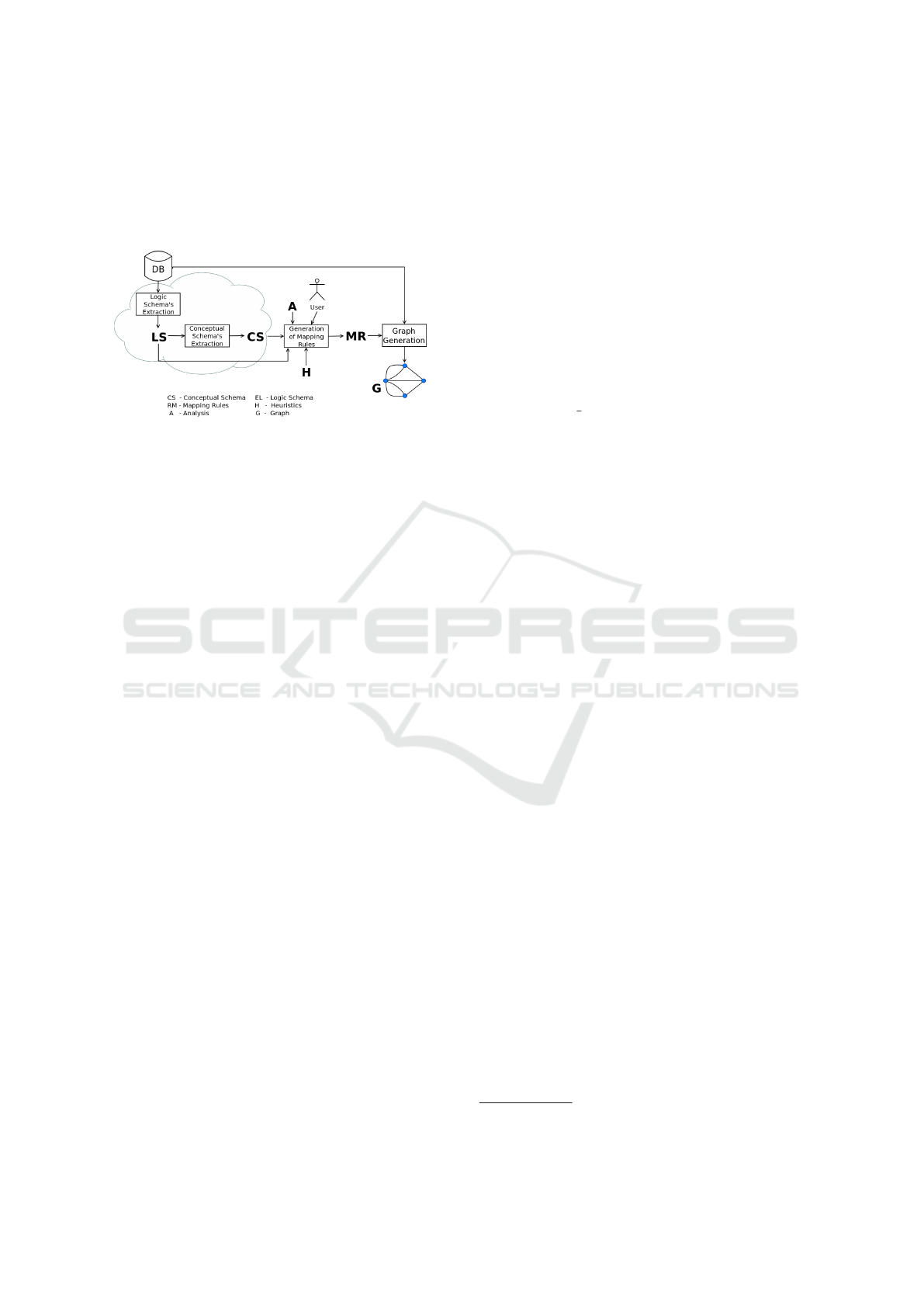
Figure 2 summarizes the proposed approach. First,
we assume that it is possible to get an ER schema
from a relational logical schema (LS) using some re-
verse engineer technique (Heuser, 2009). Sometimes
Managing Graph Modeling Alternatives for Link Prediction
73
it is difficult to get some automatic support for this
action. However, it is important to produce the ER
schema, due to its semantic richness and expressive-
ness in representing the reality. To do this, it may be
necessary to count on the domain specialists.
Figure 2: Flow chart for the proposed approach.
Then, taking the ER schema (CS), we analyze
each pair of entities (E
1
, E
2
) for which there is a re-
lationship (R), as the example in Figure 1. At this
point, the designer may consider different graph mo-
deling alternatives. The idea is to stimulate a deeper
exploration of the schema to obtain different graphs.
However, this is not an easy task, since there are many
different analysis, and besides, there are some (more
than one) graph modeling alternatives that can be ex-
plored. Therefore, the main goal of this work is to
come up with some user support. We assume that gi-
ven a set of analysis algorithms (A) and a set of heu-
ristics (H), it is possible to lead the user on choosing
a useful graph modeling. Finally, based on the user
choice, a set of mapping rules (MR) will transform
data into the desired graph (G).
To identify such heuristics, some experiments
were performed with focus on link prediction algo-
rithms. The next section describes them, as well as
their results and the extracted heuristics.
5 EXPERIMENTS AND RESULTS
5.1 Experiments Settings
For the experiments, an ordinary conceptual modeling
situation was considered, where a pair of entities
(E
1
, E
2
) is connected by only one binary relations-
hip with a multivalued attribute (see Figure 1). This
schema situation appears recurrently in database mo-
deling projects. Exploring a specific ordinary case al-
lows us to apply and compare different analysis and
metrics results. It is worth to mention that it is pos-
sible to explore the whole schema by focusing in its
parts, one at a time.
Figure 3 shows the flow chart for the heu-
ristic construction. Given a dataset (DB) and a
conceptual schema (CS), different graph modelings
(G
1
, G
2
, ..., G
n
) are generated. And for all these op-
tions, a pre-selected analysis set (A
1
, A
2
, ..., A
m
) is ap-
plied. Results have been generated from each pair
graph-analysis R
k
(G
i
, A
j
), such that (1 ≤ k ≤ n × m),
and from such results, heuristics (H) were created.
The experiments were performed over well-
known and open datasets, so it was possible and fe-
asible to check the results.
The first dataset, which we name as SMDB (Sam-
ple Movie Database), contains data about persons
(125 instances) and movies (38 instances), with a rela-
tionship “acted in” which contains a multivalued at-
tribute “role” between them. That multivalued attri-
bute means that one person may play more than one
role in the same movie.
The first experiment used intentionally a small da-
taset to easily explore the results, their impact on mo-
dels and identify some kind of pattern which can help
in creation of the heuristics. The second experiment
used a larger dataset in order to confirm the behavior
observed in the first experiment. This dataset contains
movies and actors data from TMDB
2
.
To assure some alignment between the experi-
ments, both datasets have the same domain and ER
schema, which is showed in Figure 4.
Although there are different kinds of graphs, for
this work we used the property graph, presented in
section 2.2. Our choice is laid on its wide use in the
literature.
5.2 SMDB Experiment
We have used in this experiment link prediction me-
trics among persons and movies which they acted for
a time period of twenty years in the dataset. To pre-
dict connections between persons who acted in mo-
vies and to facilitate the prediction of contemporary
actors, it was considered a restricted time window, re-
moving information about old time movies. Just per-
sons and movies between 1992 and 2012 have been
selected from the original database. Data about per-
son name and birthday; movie title, releasing data and
tagline; relationships about acting have been maintai-
ned. In this experiment Neo4j has been used to store
the dataset as a graph. To analyze and visualize the
graphs the igraph R package module was used.
We can divide this experiment in three stages.
Each stage corresponds to a variation in graph mo-
del representation. As it is possible to store informa-
tion about the data in the nodes or in the edges of the
2
http://www.themoviedb.org/
ICEIS 2018 - 20th International Conference on Enterprise Information Systems
74
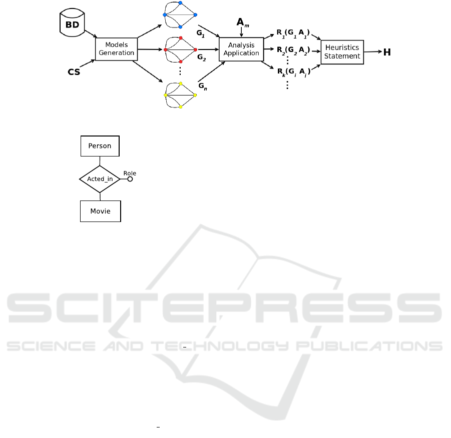
Figure 3: Flow chart for the heuristic construction.
Figure 4: ER schema for the Experiments datasets.
graph, the goal of the first two stages is to evaluate the
impact of topological changes in the link prediction
results.
In the first stage, the graph model keeps two ty-
pes of nodes and one type of relationship between
them. Nodes can be of Person or Movie type. The
Person nodes have one attribute called Name. Mo-
vie nodes have three attributes: Title, Releasing and
Tagline. The edges have just one type, Acted in, and
only one attribute, Role. Actors can have more than
one role in their attribute. Figure 5(a) shows a graph
cut-off obtained in this stage.
The second stage keeps the same information of
the graph of the first stage. However, in the second
stage there are three types of nodes: Person, Movie
and Acting. The edges of type Acted in in the first
stage (connecting Person or Movie nodes) are now re-
presented as nodes. Moreover, Acting nodes have an
attribute called Role. In this graph, nodes are con-
nected by edges with no label and no attributes. Fi-
gure 5(b) shows a graph cut-off for this stage.
The graph model of the third stage have a small
difference if compared with the second one. Nodes
and edges are of the same type and have the same at-
tributes. But, in the new graph model, Acting nodes
are split in as many nodes as there are distinct role va-
lues for the Role attribute. For instance, if some actor
has two or more roles in a movie, the acting node of
graph model 2 will be split into two or more different
nodes, each one representing a single role of the actor
in that movie. Figure 5(c) shows a cut-off of the graph
for the third stage.
Using the metrics from the analysis set it was pos-
sible to extract some predictions. Some of them were
easy to understand and easily we comprehended the
settings of each metric to suggest a new edge between
two nodes. Each metric analyzes some graph topolo-
gical information to return the predictions.
For instance, for every pair of existing nodes in
all the three graph models, it is possible to compute
the Katz coefficient (Katz is a path assembling metric
and the graphs are connected). Table 2 shows for four
pairs of nodes the Katz coefficient obtained in each
model. The analyzed pairs are Person x Person and
Movie x Movie, the only kind which are present in
every model. On the other hand, there are some pairs
of nodes that can not be analyzed in all the three mo-
dels. For instance, common neighbor metrics as Jac-
card and Adamic/Adar can not be computed for pairs
of type Person x Person or Movie x Movie in models
2 and 3.
Figure 5 illustrates the different conditions to
compute common neighbor coefficient value for each
type of pairs of nodes in the three models. For a spe-
cific pair of nodes, Hugo Weaving and Tom Hanks
(highlighted in blue), the Jaccard and Adamic/Adar
coefficients can be computed in first model, because
in the corresponding graph they share the same neig-
hbor, Cloud Atlas (Figure 5(a)). In the second model,
it is not possible to compute the last two coefficients
for this specific pair of nodes, because they do not
share common neighbors (Figure 5(b)). However, in
model 2 it is possible to compute those coefficients for
the corresponding Acting nodes (highlighted in blue).
In model 3, it is not possible to compute the Jaccard
and Adamic/Adar coefficients for the mentioned pair,
for the same reasons mentioned in model 2 (Figure
5(c)).
Another example appears in model 1. It is not
possible to compute Jaccard and Adamic/Adar coeffi-
cients for the pairs of nodes Person x Movie, because
these types of nodes are adjacent in the corresponding
graph, so they do not have common neighbors. Ho-
wever, it is possible to compute those coefficients in
models 2 and 3 for that type of pair. The same occurs
for pairs of type Person x Person and Movie x Movie.
Managing Graph Modeling Alternatives for Link Prediction
75
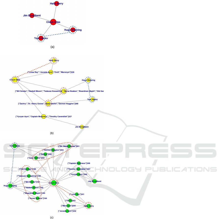
Figure 5: SMDB graph cut-off for models 1, 2 and 3.
As said before, some pairs of nodes can be used to
predict links by common neighbor based coefficients
or not, depending on the chosen model.
5.3 Heuristics
The following heuristics were identified based on the
previously reported experiment. They were stated ba-
sed on an ordinary conceptual schema situation, fre-
quently found in any domain, where a pair of entities
are connected by one binary relationship, as explained
in Section 4.
With respect to link prediction analysis, different
graph modelings allow different interpretations and
predictions. In other words, the choice of the graph
modeling and the analysis to be used on it, depends
on what it is intended to predict. The following heu-
ristics addresses this issue.
Given the conceptual schema situation represen-
ted by Figure 1, first the user needs to decide what
he wants to predict. Possible relations are: E
1i
× E
1 j
,
E
2i
× E
2 j
, E
1i
× E
2 j
, R
i
× R
j
, A
i
× A
j
, E
i
× R
j
e
E
i
× A
j
. Once prediction is defined, then just some
of the following graph modelings possibilities will
attend his need. The alternatives are:
Model 1: Instances of entities E
1
and E
2
as nodes,
instances of relationship R as edges with labels;
Model 2: Instances of entities E
1
and E
2
, and
instances of relationship R are nodes connected by
edges without labels;
Model 3: Instances of entities E
1
and E
2
, and values
of attributes A from R are nodes, which are connected
by edges without labels.
Table 1 shows the correspondence between these
three possible graph modeling, and five types of re-
lation (pairs) predictions, identifying which metrics
(Jaccard, Adamic/Adar, Katz) may be used on a mo-
del to reach a prediction.
For instance, for the first graph modeling possibi-
lity (model 1), if the user intends to predict pairs of
nodes of the same entity, E
1i
xE
1 j
or E
2i
xE
2 j
, then,
all metrics (Jaccard, Adamic/Adar and Katz) are
applicable. On the other hand, if the user intends to
predict relations between different entities, E
1i
xE
2 j
,
only path assembling predictions, such as Katz,
are applicable. Based on Table 1, more formally,
heuristics can be expressed as follows:
Heuristic 1: For predictions E
1i
× E
1 j
or E
2i
× E
2 j
:
Model 1 may be used for Jaccard, Katz and Ada-
mic/Adar analysis; Models 2 and 3 may be used only
for Katz analysis.
Heuristic 2: For predictions E
1i
× E
2 j
: Model 1 may
be used only for Katz analysis; Models 2 and 3 may
be used for Katz, Adamic/Adar and Jaccard analysis.
Heuristic 3: For predictions R
i
× R
j
: Model 2 may
be used for Katz, Adamic/Adar and Jaccard analysis.
Heuristic 4: For predictions A
i
× A
j
: Model 3 may
be used for Katz, Adamic/Adar and Jaccard analysis.
Heuristic 5: For predictions E
i
× R
j
: only Model 2
may be used for Katz analysis.
Heuristic 6: For predictions E
i
× A
j
: only Model 3
may be used for Katz analysis.
Although these heuristics are limited to three mo-
ICEIS 2018 - 20th International Conference on Enterprise Information Systems
76

deling alternatives, and three distinct prediction ana-
lysis, they can be extended. Other modeling alternati-
ves and prediction analysis can be addressed.
5.4 TMDB Experiment
Aiming to confirm the previous experiment results,
new experiments have been made using a greater da-
taset with the same previous analysis. A subset from
the original set has been extracted, where movies and
actors refer to “Crime” movies. The TMDB experi-
ment used the same data schema of the last experi-
ment. To assure the link prediction it was considered
the largest connected component from the modeled
graph of each modeling. The obtained graph for the
first model has 4486 nodes and 5046 edges. The se-
cond model graph has 9532 nodes and 10092 edges.
And the last and third model graph has 9561 nodes
and 10150 edges.
The goal of this experiment is to assure if the
recognized behaviors from previous experiment are
the same for a largest dataset. Results showed that
the same patterns were found, confirming the heu-
ristics. In addition, it was possible to evaluate the
gains quantitatively (Section 5.4.1) and qualitatively
(Section 5.4.2), as follows. First we show a quantita-
tive analysis highlighting the richness of results that
we can get with the different modelings. Then, we
proceed with a qualitative analysis in order to illus-
trate the usefulness of this approach.
5.4.1 Quantitative Analysis
First we focus the analysis on Katz results, because
this coefficient allowed us to compare the three mo-
deling alternatives.
The types of node pairs suggested by Katz were
the same for each model as in Section 5.2. Note that
in Table 2, the coefficient value for a specific pair of
nodes, obtained for model 1 is greater than for the ot-
her models. Similarly, this behavior occurred in the
second experiment. This is due to the fact that mo-
dels 2 and 3 are bigger than model 1, in terms of the
number of nodes and edges, which makes the Katz
coefficient values to be diluted in those models.
Table 3 shows the number of suggested pairs
for each model using Katz coefficient. It is worth
to mention that models 2 and 3 provide much more
pairs than model 1. Besides, as mentioned before,
they also provide new types of pairs such as Movie
x Acting and Acting x Acting for model 2, and Role
x Role and Movie x Role for model 3, enriching the
results.
In order to perform a more strict analysis, we
chose to focus on the best ranked results. Therefore,
we established a threshold with the following value 1
x 10
−5
, based on value variation when using model 1.
Using this threshold, Table 4 shows that 14% of the
pairs were selected from those suggested for model 1
in Table 3, and 1.19% and 1.16% were selected for
models 2 and 3, respectively.
Differently from what shows Table 3, the total
number of suggested pairs shown in Table 4, is gre-
ater for model 1 than for models 2 and 3. However,
the variety of node types is greater for models 2 and 3
than model 1, showing richer results.
Now let us analyze the best ranked types of pairs
in the context of the three coefficients. According to
Tables 5, 6 and 7, it is possible to identify different
types of pairs in the top positions for model 1. Note
that for Jaccard (Table 5) the pair Person x Person is
the best ranked, while for Adamic/Adar (Table 6) the
pair Movie x Movie is the best, and finally for Katz
(Table 7) the best pairs are Movie x Person. The rea-
son of this different behavior is related to the nature of
the coefficients. For instance, since in this model the
graph has edges between Actor and Movie nodes, the
greatest value for Jaccard can happen in two cases:
1. When two actors acted only in the same movies
and no other movie separately, and
2. When two distinct movies have exactly the same
casting.
Case (i) is more probable to happen, because it is
more difficult that two movies have the same casting.
Adamic/Adar also works with common neighbors
as Jaccard. However it penalizes the pair when its
common neighbors are highly connected. For in-
stance, if two actors have many movies in common,
but these movies have a high number of connections
to other actors, this pair is not so significant for Ada-
mic/Adar than for Jaccard. Different from Jaccard,
for Adamic/Adar, some pairs of movies will probably
be shown in the top positions of the ranking. Typi-
cally, these are movies with just a few common neig-
hbors (actors), which do not participate in many other
movies. Table 6 shows the five top movie pairs that
have this characteristic.
Therefore, according to the user needs, i.e. type
of pairs, the right analysis should be chosen, or yet,
results could complement each other.
As said before, the Katz ranking (Table 7) differs
from the other rankings. It prioritizes pairs of nodes
connected by short length paths in the graph. The best
ranked suggestions are pairs Movie × Person, already
linked by an edge in the graph.
Managing Graph Modeling Alternatives for Link Prediction
77

Table 1: Suggested pairs of nodes for all coefficients.
E
1i
× E
1 j
E
2i
× E
2 j
E
1i
× E
2 j
R
i
× R
j
A
i
× A
j
E
i
× R
j
E
i
× A
j
Model 1
Jaccard, Katz,
Adamic/Adar
Jaccard, Katz,
Adamic/Adar
Katz - - - -
Model 2 Katz Katz
Jaccard, Katz,
Adamic/Adar
Jaccard, Katz,
Adamic/Adar
- Katz -
Model 3 Katz Katz
Jaccard, Katz,
Adamic/Adar
-
Jaccard, Katz,
Adamic/Adar
- Katz
Table 2: Katz coefficients for suggested pairs for 3 models
in SMDB dataset (enclosed in brackets the ranking of each
pair Person x Person and Movie x Movie).
Model 1 Model 2 Model 3
Tom Hanks x Meg Ryan 0.188 - [363] 0.006 - [4239] 0.023 - [4629]
Tom Hanks x Bill Paxton 0.196 - [360] 0.006 - [4247] 0.022 - [4635]
The Matrix x
The Matrix Reloaded
0.295 - [110] 0.009 - [4030] 0.010 - [6766]
Apollo 13 x
The Polar Express
0.089 - [543] 0.002 - [5246] 0.075 - [2524]
Table 3: Number of suggested pairs for each model with
Katz in TMDB dataset.
Model 1 Model 2 Model 3
Person x Person 6.546.771 6.514.245 6.514.246
Person x Movie 1.353.506 1.332.090 1.332.090
Movie x Movie 69.751 67.896 67.896
Movie x Acting - 1.485.963 -
Movie x Role - - 1.497.033
Acting x Acting - 8.106.351 -
Role x Role - - 8.227.596
Person x Acting - 14.537.471 -
Person x Role - - 14.645.770
Total 7.970.028 32.044.016 32.284.631
Table 4: Number of suggested pairs for each model with
threshold 1 x 10
−5
in TMDB dataset.
Model 1 Model 2 Model 3
Person x Person 1.049.949 32.573 21.677
Person x Movie 328.262 17.340 17.977
Movie x Movie 31.307 1.431 1.431
Movie x Acting - 40.191 -
Movie x Role - - 40.195
Acting x Acting - 168.672 -
Role x Role - - 171.996
Person x Action - 124.114 -
Person x Role - - 124.385
Total 1.409.518 384.321 377.661
Table 5: Jaccard ranking for Model 1 in TMDB dataset.
Model 1
Tony Kendall x Gert Gnther Hoffmann 0,875
Gert Gnther Hoffmann x Brad Harris 0,875
Heinz Weiss x George Nader 0,875
Stringer Davis x Charles ’Bud’ Tingwell 0,8
Charles ’Bud’ Tingwell x Margaret Rutherford 0,8
John Randolph Jones x Udo Kier 0,666
5.4.2 Qualitative Analysis
Because of the richness of TMDB dataset, it was
possible to get new interpretations for the results.
Table 6: Adamic/Adar ranking for Model 1 in TMDB data-
set.
Model 1
Beck - Flickan x Beck - Den japanska 9,566
Dancer in the Dark x Dogville 7,402
The Spider Woman x The Adv. of Sherlock Holmes 5,770
36 x The Last Deadly Mission 5,770
Gert Frobe x Wolfgang Preiss 2,252
Table 7: Katz ranking for Model 1 in TMDB dataset.
Model 1
Armin Mueller Stahl x Angels & Demons 13,33247
Stellan Skarsgrd x Angels & Demons 13,22136
Carmen Argenziano x Angels & Demons 12,31250
Tom Hanks x Angels & Demons 12,25930
Elya Baskin x Angels & Demons 12,24942
Instead of analyzing the rankings for each model, we
selected some specific suggestions of pairs and have
compared the results that could be obtained with the
different analysis. For instance, to answer the query
which movies are similar, we focused on the Movie
× Movie pair type. Table 8, for Model 1, shows
5 suggested pairs using Katz analysis, which are
different from those suggested using Adamic/Adar,
showed on Table 6. It is worth mention that the bro-
ader nature of Katz analysis enabled to get different
and complementary results.
Table 8: Katz rankings for pairs Movie × Movie of three
models in TMDB dataset.
Model 1 Value
Angels & Demons x Dogville 3,9847
Angels & Demons x Dancer in the Dark 3,3753
Angels & Demons x Identity 2,6619
Angels & Demons x The Green Mile 2,2638
Angels & Demons x The Name of the Rose 2,1899
Model 2 Value
Angels & Demons x Dogville 0,0105
Angels & Demons x Dancer in the Dark 0,0088
Angels & Demons x Identity 0,0087
Angels & Demons x The Name of the Rose 0,0073
Angels & Demons x Eastern Promises 0,0072
Model 3 Value
Angels & Demons x Dogville 0,0105
Angels & Demons x Dancer in the Dark 0,0088
Angels & Demons x Identity 0,0087
Angels & Demons x The Name of the Rose 0,0073
Angels & Demons x Eastern Promises 0,0072
ICEIS 2018 - 20th International Conference on Enterprise Information Systems
78

Moreover, it was observed (on Table 8) that Katz
analysis results were almost the same for the three
models. At a first look, we might think that models
2 and 3 are not useful. However, remember that with
them, it is possible to get different suggested types of
pairs, besides the Movie × Movie pairs. For instance,
we can answer the following question: what roles can
we suggest for a specific actor/actress?. This ques-
tion can be answered by Katz analysis on models 2
and 3. Let us focus on pairs Person × Role suggested
by Katz on model 3. If we take Joe Pesci as a refe-
rence actor, which roles could be close to him, and
maybe a good suggestion for a future movie part? To
do this, we need to discard Katz analysis top ranked
results, and take just results which include Joe Pesci
own roles (movies in which he acted). The subsequent
top ranked pairs bring roles from Joe Pesci neighbor-
hood. These roles are from actors he co-acted with,
or even more distant ones. For example, we could
take from the ranking, some pairs Person × Role with
Joe Pesci as person and roles from Robert De Niro
(such as Father Bob and Travis Bickle), and from Tom
Hanks (such as Robert Langdon and Paul Edgecomb).
See in Table 9 the corresponding coefficient for these
pairs. We observe that Joe Pesci take part in 4 movies
with Robert De Niro, whereas Joe Pesci never acted in
the same movie with Tom Hanks, considering infor-
mation in our dataset. Observe that actors that acted in
common movies has Katz coefficient greater (for in-
stance, Joe Pesci and Robert De Niro). This fact can
be useful when looking for actors that are able to play
a specific role, or when looking for a replacement for
an actor.
Table 9: Katz results for pairs Person × Role with Joe Pesci
in TMDB dataset.
Pair Model 3
Joe Pesci x Father Bobby 2,909633e-04
Joe Pesci x Travis Bickle 2,902883e-04
Joe Pesci x Robert Langdon 9,878335e-09
Joe Pesci x Paul Edgecomb 1,757311e-10
Another interesting observation is when we com-
pare again pairs Person × Role and consider the role
Frank Sparks played by actor William Forsythe. The
Katz coefficient for the pair Joe Pesci × Frank Sparks
is 6,64497e-05, lower than the coefficient for the pair
Joe Pesci × Father Bobby. We can observe that there
are shortest paths with the same length between the
nodes Joe Pesci and Father Bobby and between the
nodes Joe Pesci and Frank Sparks in the associated
graph, but Katz coefficient is greater for the pair Joe
Pesci and Father Bobby because exist more than one
shortest path between them.
6 CONCLUSION AND FUTURE
WORKS
This work addressed the task of mapping relational
data into graph representation. It proposes a set of
heuristics, aiming to help the user to model a graph.
We highlight that even with a set of analysis coeffi-
cients in hands, before applying them, it is necessary
to acknowledge the conceptual and logical schema
from Relational Databases to better understand the
data and the prediction intention, and thus reach a
well modeled graph.
Initial experiments were reported and enabled to
identify a set of heuristics. These experiments focu-
sed on topological analysis. They applied three link
prediction metrics over two different datasets: SMDB
(a toy example) and TMDB. However, additional ex-
periments are needed, using datasets from different
domains, and a larger set of analytical coefficients, in
order to validate or maybe extend these heuristics.
Finally, in the reported experiments, we focu-
sed only on the binary relationship modeling con-
struct. Although this is an ordinary conceptual mo-
deling construct, that appears recurrently in many da-
tabase modeling projects, we plan to use other mo-
deling constructs, such as n-ary relationships, specia-
lization/generalization, and aggregation.
REFERENCES
Aggarwal, C. C. (2011). Social Network Data Analytics.
Springer Publishing Company, Incorporated, 1st edi-
tion.
Bizer, C. (2003). D2R MAP - A database to RDF mapping
language. In Proc. of the Twelfth Intern. World Wide
Web Conf. - Posters, WWW 2003, Budapest, Hungary,
2003.
Bordoloi, S. and Kalita, B. (2013). Designing graph data-
base models from existing relational databases. Int. J.
of Computer Applications, 74(1):25–31.
Chen, P. P.-S. (1976). The entity-relationship model;toward
a unified view of data. ACM Trans. Database Syst.,
pages 9–36.
Codd, E. F. (1970). A relational model of data for large
shared data banks. Commun. ACM, pages 377–387.
Easley, D. and Kleinberg, J. (2010). Networks, Crowds,
and Markets: Reasoning About a Highly Connected
World. Cambridge University Press, New York, NY,
USA.
Heuser, C. (2009). Projeto de banco de dados : Volume 4 da
S
´
erie Livros did
´
aticos inform
´
atica UFRGS. Bookman.
Jindal, A., Rawlani, P., Wu, E., Madden, S., Deshpande, A.,
and Stonebraker, M. (2014). Vertexica: Your relatio-
nal friend for graph analytics! Proc. VLDB Endow.,
7(13):1669–1672.
Managing Graph Modeling Alternatives for Link Prediction
79

Liben-Nowell, D. and Kleinberg, J. (2007). The link-
prediction problem for social networks. Journal of
the American Soc. for Inf. Sci. and Tech., pages 1019–
1031.
Rodriguez, M. A. and Neubauer, P. (2010). Constructions
from dots and lines. Bulletin of the American Society
for Information Science and Technology, 36(6):35–41.
Simmen, D., Schnaitter, K., Davis, J., He, Y., Lohariwala,
S., Mysore, A., Shenoi, V., Tan, M., and Xiao, Y.
(2014). Large-scale graph analytics in aster 6: Brin-
ging context to big data discovery. Proc. VLDB En-
dow., 7(13):1405–1416.
Virgilio, R. D., Maccioni, A., and Torlone, R. (2014a). Con-
verting relational to graph databases. In First Interna-
tional Workshop on Graph Data Management Expe-
riences and Systems.
Virgilio, R. D., Maccioni, A., and Torlone, R. (2014b).
Model-driven design of graph databases. In Concep-
tual Modeling: 33rd International Conference, ER
2014, Atlanta, GA, USA, October 27-29, 2014. Pro-
ceedings, pages 172–185.
Wardani, D. W. and Kng, J. (2014). Semantic mapping re-
lational to graph model. In Computer, Control, Infor-
matics and Its App., 2014, pages 160–165.
Xirogiannopoulos, K., Khurana, U., and Deshpande, A.
(2015). Graphgen: Exploring interesting graphs in re-
lational data. PVLDB, 8(12):2032–2043.
Xirogiannopoulos, K., Srinivas, V., and Deshpande, A.
(2017). Graphgen: Adaptive graph processing using
relational databases. In Proceedings of the Fifth Inter-
national Workshop on Graph Data-management Ex-
periences & Systems, GRADES’17, pages 9:1–9:7,
New York, NY, USA. ACM.
ICEIS 2018 - 20th International Conference on Enterprise Information Systems
80
