Bus Schedule Rationalisation

An Analysis of Trip Completion Times

Shankar Venkatagiri

, Gaurav Kumar

and Munish Kaushik

Indian Institute of Management Bangalore, India

IBM India Private Limited, India

Keywords:

Vehicle Analytics, AVL Systems, ITS, Time Series Modeling, Dashboard Visualisation, Big Data Platforms.

Abstract:

Public transit systems offer a smart option to reduce congestion in Indian cities. Due to the poor service quality

of public bus transit operators, more commutes are now being completed using private transport, exacerbating

trafﬁc problems. In this paper, we examine AVL data generated by public buses in Bengaluru and identify a

problem of schedule compliance for buses plying a popular route. We then undertake a time series analysis of

the trip run times. We ﬁnalise on an ARIMA model and derive a forecast of completion times. We conclude

with recommendations for trip scheduling.

1 INTRODUCTION

One-thirds of India's population lives in dense ur-

ban agglomerations (UA). The transit modal share

varies from UA to UA. Citizens in most UAs can

access public transit modes such as auto rickshaws

and buses; larger UAs maintain commuter trains and

metro rail services. Bengaluru is India's fourth largest

UA, with a population of 10 million. Over the past

three decades, a prosperous IT industry has brought a

steady inﬂux of workers into the city. Business parks

and residential areas located on the periphery have ex-

panded the size of the city to 700 sqkm. Sweeping in-

frastructural changes are frequently made to accom-

modate the increased use of privately owned vehicles

that often transport a lone passenger and contribute to

widespread congestion.

Public transit services in India have their share of

problems (Badami and Haider, 2007). After devising

metrics that are appropriate to this context, Badami

and Haider compare the performance of bus services

across various UAs. Their analysis shows that rid-

ership numbers have steadily fallen over time. They

highlight a “viability-affordability dilemma”: faced

with mounting expenses, transit operators are forced

to hike fares, which causes ridership to decline.

Unreliable arrival times and overcrowding are

other factors that make commuters switch to using

private vehicles. With the objective to plan services

more effectively, public transit operators have begun

to invest in technologies such as automatic passenger

counters (APC) and automatic vehicle location (AVL)

systems. However, only a select few have developed

the capabilities to process the large volumes of col-

lected data. A strong decision support tool can factil-

tate effective trip scheduling and monitoring, mainte-

nance management, trend analysis and a host of other

activities (Furth et al., 2003).

Trafﬁc in Indian UAs is vastly heterogeneous;

buses and heavy vehicles jostle for space with two-

, three- and four-wheelers on congested roads. Lane

discipline is not maintained. Arterial roads are peren-

nially under repair. Trafﬁc signals malfunction. These

factors invalidate the simplifying assumptions made

by most transportation models. Statistical analyses

with time-location data can generate more actionable

insights (Vanajakshi et al., 2009).

Trip completion or run time is a key consideration

for commuters deciding on their mode of transit. Reli-

able run time estimates are critical for a transit opera-

tor to build and display “rational” schedules and retain

ridership. AVL and APC data have been harnessed to

estimate trip run times in a predictable trafﬁc setting

etreault and El-Geneidy, 2010).

We shall take up the complex problem of run

time estimation in an Indian context, by examining

a popular all-day bus route operated by Bengaluru

Metropolitan Transport Corporation (BMTC). Our

analysis shows that a seasonal ARIMA model best ﬁts

the trip completion data, and can be used by schedule

planners to arrive at reliable timetables.

The paper is organised as follows. Section 2 high-

Venkatagiri, S., Kumar, G. and Kaushik, M.

Bus Schedule Rationalisation.

DOI: 10.5220/0006711904030410

In Proceedings of the 4th International Conference on Vehicle Technology and Intelligent Transport Systems (VEHITS 2018), pages 403-410

ISBN: 978-989-758-293-6

403

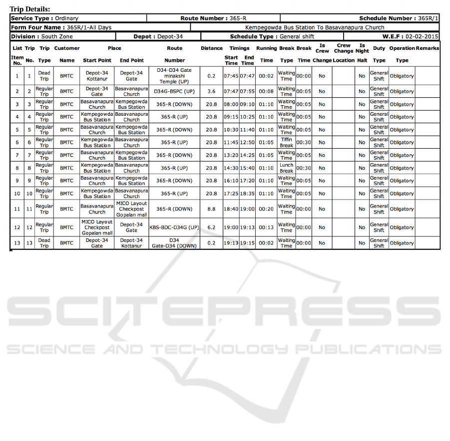
Figure 1: Example Form IV Schedule.

lights some operational realities at BMTC. Section 3

details the intelligent transportation system (ITS) un-

der implementation, and computing infrastructure to

further process the data. Section 4 exposes the prob-

lem of trip run time variance, which impacts schedule

compliance. Using techniques from time series analy-

sis, we model the run times in Section 5, and compare

model accuracies. The paper concludes with some di-

rections for investigation.

2 OPERATIONAL CONTEXT

The Bengaluru Metropolitan Transport Corporation

(BMTC) is the city's sole public bus transit provider.

Its 6,400-strong ﬂeet services the needs of commuters

travelling to urban and suburban areas. Each day, the

ﬂeet completes 75,000 trips and covers 1.15 million

service km. By facilitating 5 million rides, these buses

cater to 40% of the city's demand. BMTCs premium

services, which have been in operation since 2006,

comprise 10% of the ﬂeet. These services are efﬁcient

and somewhat proﬁtable (Hanumappa et al., 2016).

Every bus follows a designated schedule termed as

Form-IV, which lists the speciﬁc up and down trips to

be covered on a route (Figure 1). Created years ago,

these schedules have remained unchanged, whereas

trafﬁc on Bengaluru's roads has increased manifold.

This has led to signiﬁcant deviations from the Form

IV stipulation as well as revenue projections. Occa-

sionally, drivers rushing to complete their schedule

tend to commit serious mistakes.

BMTC management has responded by prioritising

the rationalisation of its Form-IVs, which number a

formidable 6,100. The new schedules must take into

account variations in the trafﬁc conditions, which are

governed by a diverse set of parameters such as the

month, day of week, time of day and whether or not it

is a holiday. The pivotal role of trip run time estima-

tion in this exercise is fairly obvious.

2.1 Objective of our Study

It is our mission to assist planners at BMTC with

drawing up rational schedules. The ﬁrst step would

be to examine trip run patterns in order to arrive at

reliable estimates. By “piecing together” these esti-

mates for the up and down trips, we can decide on a

workable number to include in the schedule.

For our research, we choose Schedule 365R,

whose trips run all day along a route of 21 km, con-

necting a national park on the outskirts of Bengaluru

with the hub for BMTC in the city centre. Figure 2

lists the main bus stops for this route. On weekdays,

trips are delayed anywhere between 10 to 60 minutes.

Since peak hour kicks in by 8:30 a.m., we choose to

investigate Trip 3, which is scheduled to run between

8:00 a.m and 9:10 am (see Figure 1).

VEHITS 2018 - 4th International Conference on Vehicle Technology and Intelligent Transport Systems

404

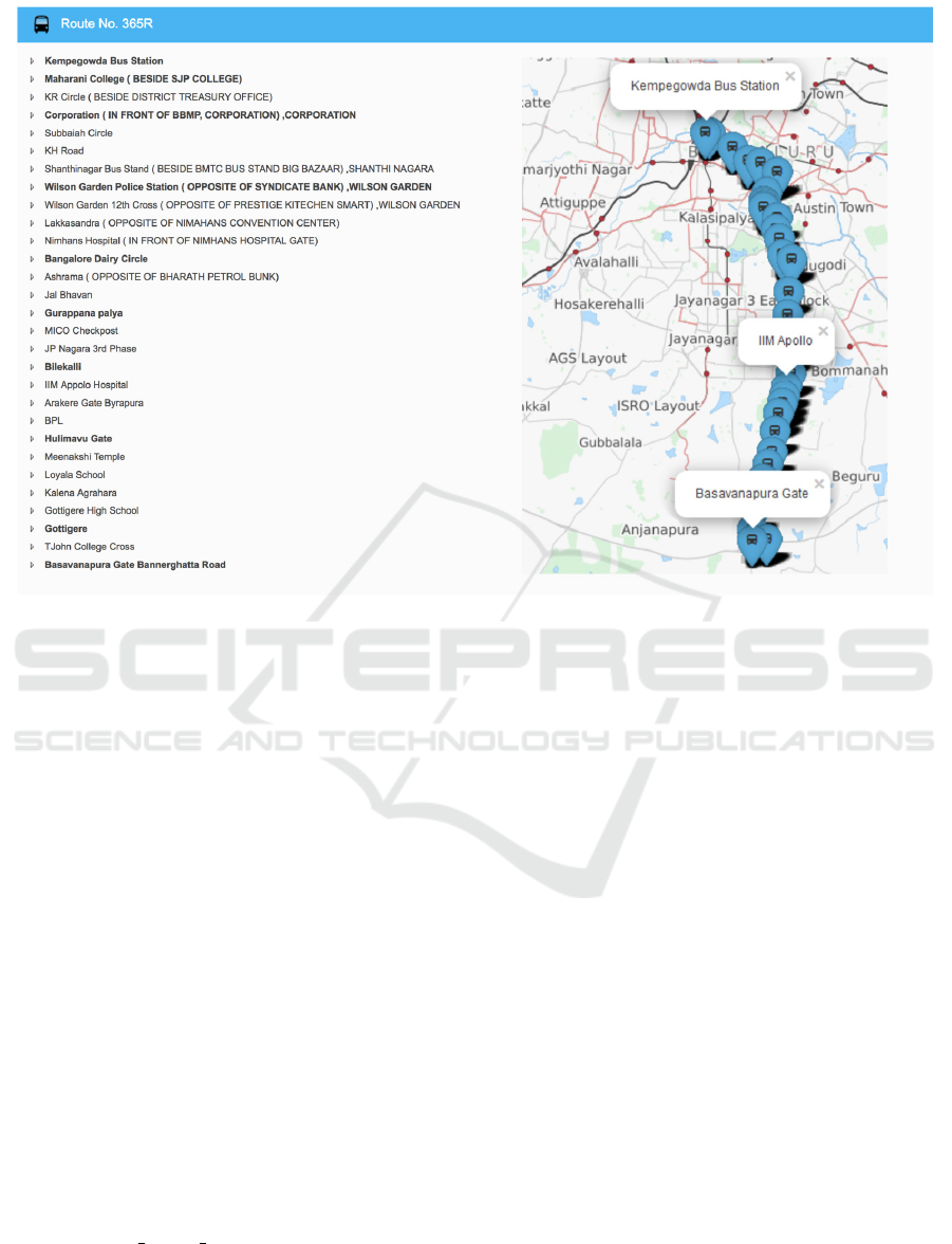
Figure 2: Bus Stops on Route 365R.

3 ITS AT BMTC

In what was a ﬁrst for Indian public transit opera-

tors, BMTC launched a comprehensive ITS initiative

in June 2016. Vehicle tracking units (VTU) have been

installed on all buses, and are successfully relaying

their latitude-longitude coordinates every 10 seconds

via GPS to a central ITS server. Conductors have been

relaying their ticket sales using GPS-enabled Elec-

tronic Ticketing Machines (ETMs). Staff who are sta-

tioned at a Control Centre can now track buses in real

time, and attend to any emergencies.

3.1 Data Collection

On a given duty date, a bus makes multiple trips. The

conductor uses the ETM to key in the schedule and

trip number, as well as the start and end times for the

trip. The ITS stores all of this information in the way-

bill table (Figure 3). The VTU on-board the bus peri-

odically reports a device ID and a geo-location, along

with a timestamp, all of which are recorded in a sep-

arate table (vts parse data). The remaining tables

contain reference data for schedules, routes, bus stops

and bus to GPS device associations.

3.2 Processing Infrastructure

Whereas the waybill table receives two million up-

dates each month corresponding to the 75,000 trips

made everyday, the geo-location data relayed every

10 seconds generate close to a billion updates to the

VTS table each month. All of this data is transferred

from the production ITS server to a 10-node Hadoop

Distributed File System (HDFS) cluster, which runs a

SQL-friendly Hive database. We use a Python/Spark

program to query this database and generate a time

series of trip completion times. We then avail of

the strong support by the R platform for time series

modelling and visualisation, using packages like xts,

forecast, ggplot.

3.3 Missing Data

There are a few instances in which trip data have

gone missing; this may be attributed to worker strikes,

trip truncation, absence of service (formally termed

as missed trips) and a simple lack of records. We

have chosen to impute the missing data with the aver-

age of times taken for “neighbouring” trips that cor-

respond to the same weekday. We then obtain a con-

tiguous time frame of four months between August-

November 2016 (Figure 4).

Bus Schedule Rationalisation

405

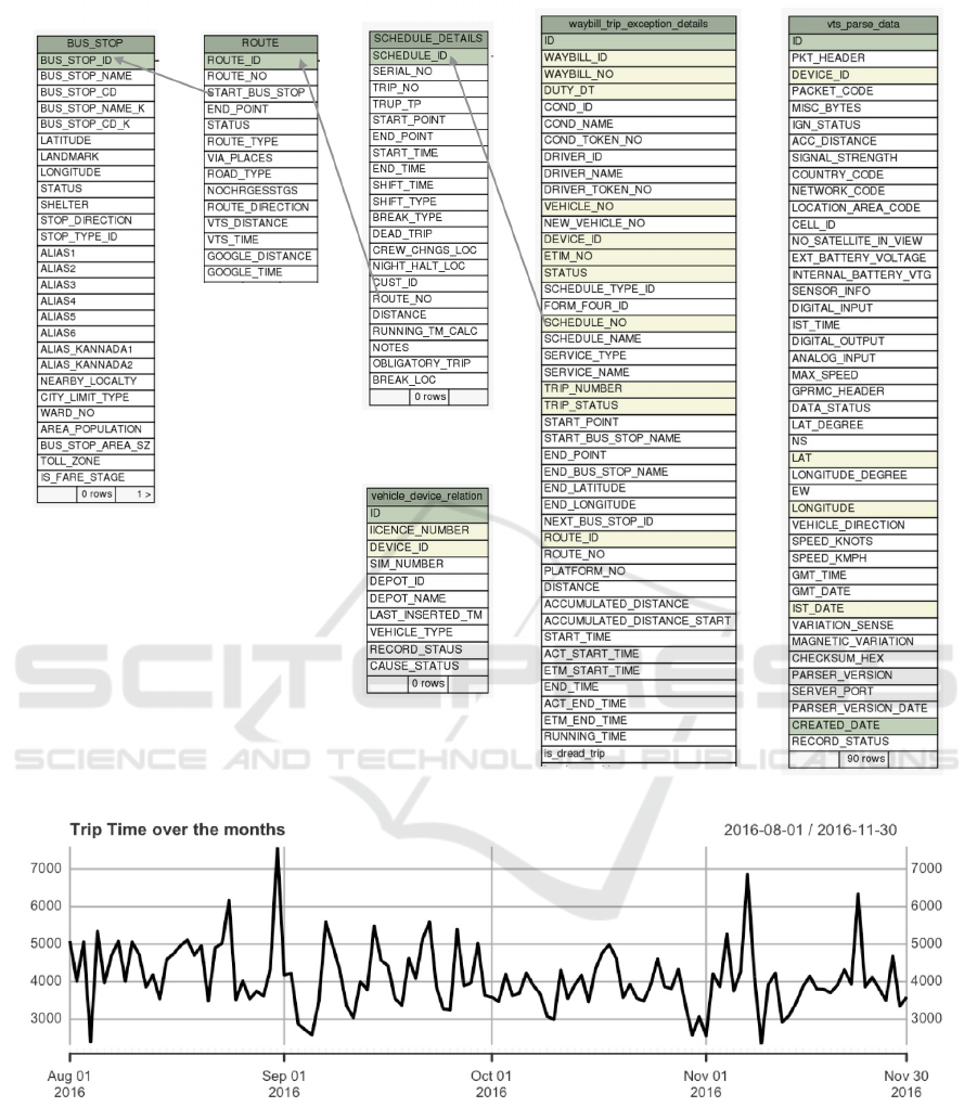
Figure 3: Excerpt of the Database Schema.

Figure 4: Completion times for Trip 3 of schedule 365R.

3.4 Unlinked Information

In the existing setup, neither the VTU nor the ETM

performs any pre-processing steps; both devices sim-

ply relay the data they gather to the ITS server. This

can be problematic. The speciﬁc trip number of the

schedule that a bus is plying on is unavailable, and

must be separately ascertained. Anomalies can arise

due to a bus missing one or more stops en route, mak-

ing incomplete trips, or skipping a trip altogether.

These events are not ﬂagged. Finally, there is no

record of events such as arrivals of a bus at the des-

ignated stops along its route and more critically, the

times of arrival; these issues hinder trip analysis.

VEHITS 2018 - 4th International Conference on Vehicle Technology and Intelligent Transport Systems

406

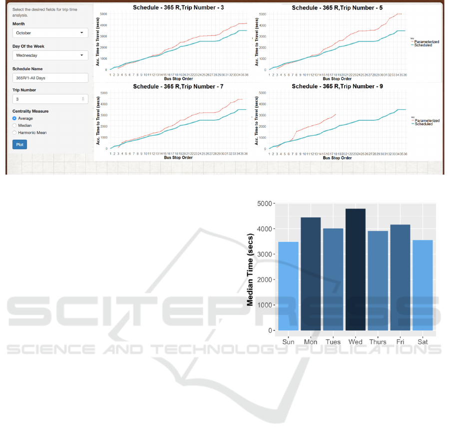
Figure 5: Average run times for Wednesdays in October 2016.

3.5 Trip Reconstruction

We make intensive use of the VTS data to reconstruct

the trips. We employ a geo-fence of ﬁxed radius to de-

tect the presence of a bus at or near a designated stop,

on the basis of its recorded lat-long values. Whereas a

liberal value for the radius could indicate that a bus is

present at multiple stops, too tight a setting could re-

sult in transits through bus stops not being detected. A

smaller geo-fence radius is advantageous; the arrival

time at a bus stop is accurately derived, and there is

reduced chance of multiple observations lying within

a single fence. For each trip, we consult the waybill

to determine the start and end times entered via the

ETM, and add a relaxation to compensate for lags in

data entry. We use this time window to extract rows

that are relevant to the trip from the VTS table. In or-

der to determine the sequence of halts, one approach

would be to take each recorded lat-long value, and

check if it falls within the geo-fence of a bus stop

on the route. This is where parallelised computations

prove to be handy.

4 SCHEDULE VARIANCE

Examine the Form IV for our chosen schedule in Fig-

ure 1. On an ordinary service day, Trip 3 must be

completed within 70 minutes. The ITS data reveals

that this is not always the case; at 4,100 seconds the

observed average for the 4 month period is less than

the stipulated time. However, the run times show a

wide variation between 2,300 and 7,600 seconds, with

a standard deviation of 860 seconds.

Figure 6 depicts the overall variation in run times,

which hints at possible delays. For instance, median

levels for Trip 3 on Monday and Wednesday far ex-

Figure 6: Variation in Trip 3 run times.

ceed the stipulated 70 minutes. Such delays might

have a cascading effect on remaining trips for the day,

leading to a fall in the total number of trips. Con-

versely, the median run time for Sunday is vastly

lower than 70 minutes; examining the actual data re-

veals that all 13 trips are completed on Sundays.

We have built a dashboard using the Shiny pack-

age of R to interactively visualize trips and transit

events, by applying ﬁlters such as month, day of week

and trip number (Figure 5). Ignoring the ﬁrst and ﬁnal

dead trips in Figure 1, 11 trips have to be completed.

However, Figure 5 makes it clear that Trips 9 and 10

are usually missed on Wednesdays; these are expected

to cover the full route of 20.8 km. Trip 9 in Figure 5

(in red) is actually Trip 11 in the Form IV listing, with

a run distance of 8.8 km.

5 ANALYSIS OF RUN TIMES

Planners would beneﬁt from a prediction model for

trip completion times that takes into account com-

Bus Schedule Rationalisation

407

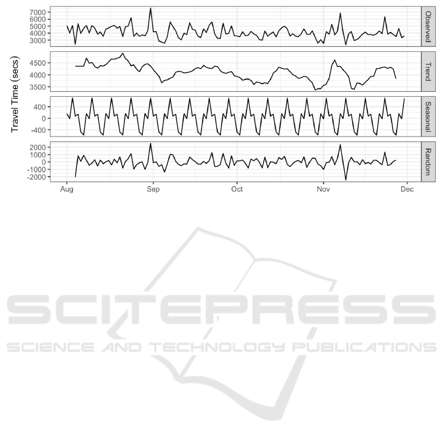
Figure 7: Completion times for trip 3 of schedule 365R.

plex trafﬁc conditions. With the reconstructed trip

data, we now undertake a systematic analysis using

techniques from time series analysis (Hyndman and

Athanasopoulos, 2014). Our training dataset consists

of trip run times for the ﬁrst 16 weeks; the models

are then validated against the ﬁnal week of November

2016.

5.1 Characterisation

Despite wide variations in run times across the week

(Figure 6), one would expect that they will demon-

strate a fair amount of seasonality; one Monday's traf-

ﬁc pattern would be comparable to another Monday's,

barring exceptions like holidays.

We shall employ an additive decomposition for

the run times (Figure 7) because the magnitude of the

seasonal ﬂuctuations around the trend cycle is unaf-

fected by the level of the time series. Barring the

peaks in September and November, the time series

appears to be stationary; this is attested by an Aug-

mented Dickey-Fuller test (p < 0.01). The trend cy-

cle for the period follows no predictable pattern. It

is clear that there is weekly seasonality. The random

signal has the characteristics of white noise.

5.2 Modelling

The peaks and troughs in the series fail to show any

regularity. Consequently, a seasonal-naive model ﬁt

with frequency = 7 results in an inaccurate forecast

(Figure 8a). The 7-day moving average ﬁt captures

the trend in the series (Figure 8b), but misses the

amplitudinal variations. Both of these ﬁts are unus-

able by schedule planners. A better ﬁt is achieved by

a Holt-Winters model with damping, which captures

the trend as well as seasonal variation (Figure 8c). It

is still insensitive to high swings.

Because travel times on corresponding weekdays

are correlated, we shall seek a seasonal ARIMA ﬁt.

The auto.arima utility in R exhaustively searches

the space of ARIMA models with lags p (for AR) and

q (for MA) of up to 5. The algorithm settles on an

ARIMA model ﬁt with trend-differencing.

ARIMA(1,1,1)(1,0,1)[7]

ar1 ma1 sar1 sma1

0.1818 -0.9829 0.7948 -0.5321

s.e. 0.0965 0.0241 0.1583 0.2278

The coefﬁcient of MA in this model is close to

unity, which is undesirable. The trend in the series

being unpredictable, we shall choose to ignore it and

drop the differencing. We shall model using seasonal

differencing alone, and obtain the ﬁt shown below.

ARIMA(1,0,1)(1,1,1)[7]

ar1 ma1 sar1 sma1

0.1847 0.0241 0.1812 -0.8282

s.e. 0.4225 0.4255 0.1572 0.1254

The residuals turn out to be normally distributed,

indicative of white noise. Carrying out a Ljung-Box

test on this new model, we conclude that the residuals

are also not correlated (with p = 0.55).

Table 1 lists a set of standard measures used to

compare the models. The Holt-Winters and ARIMA

models outperform the base naive model on all met-

rics; MASE values less than 1 suggest that forecasts

made using either of these models perform better than

the naive model.

VEHITS 2018 - 4th International Conference on Vehicle Technology and Intelligent Transport Systems

408

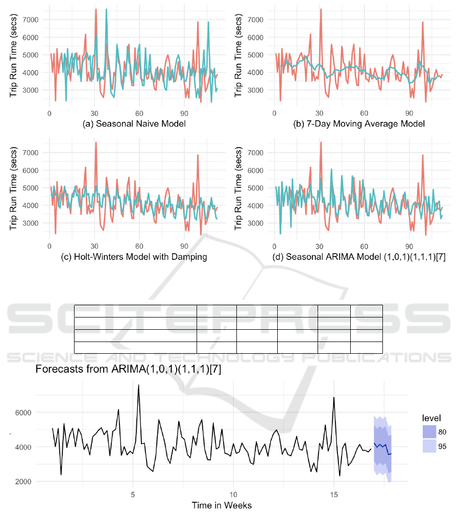
Figure 8: Different Models of the Trip Run Times.

Table 1: Comparison of Model Accuracies.

Model RMSE MAPE MASE AIC BIC

Seasonal Naive 982 18.4 1 - -

Holt-Winters (damped) 758 14.18 0.75 2039 2075

ARIMA(1, 0, 1)(1, 1, 1)[7] 772 14.16 0.76 1717 1730

Figure 9: Forecast from the Final Model.

We ﬁnalise on an ARIMA(1,0,1)(1,1,1)[7] model,

which has the lowest criterion values (AIC and BIC).

5.3 Forecast

We use the ﬁnal model to forecast trip run times; the

results are depicted in Figure 9. Planners may choose

to build their schedules on a rolling basis using the

80% conﬁdence level. The MAPE calculated for the

testing data at 20.7% is higher than the 14.16% corre-

sponding to the training data.

6 CONCLUSIONS

This paper goes over common problems that impact

bus transit authorities in the crowded cities of India.

Bus Schedule Rationalisation

409

Given the trafﬁc congestion and pollution, it is imper-

ative to explore ways in which commutes using pri-

vate vehicles can be reduced. A sizeable segment of

the citizenry would take to buses if their quality of

service could be improved. Large schedule variance

and unpredictable arrival times have had a negative

impact on commuters seeking predictable transits. In

2016, BMTC, which is Bengaluru's public bus trans-

port provider, invested in an ITS platform to capture

large volumes of AVL and ETM data generated by its

ﬂeet of 6,400 buses. The paper throws light on how

this data is stored and processed in a cluster of ma-

chines that are enabled by big data technologies such

as Spark/Hadoop/Python/R.

For our study, we select a popular route (356R) of

BMTC, and examine Trip 3 on the schedule, which

operates during the peak hours of the morning. By

querying the AVL and ETM data, we ascertain run

times for this trip over a 4 month period. Our analysis

exposes a problem of schedule variance. To suggest

remedies to this problem, we undertake a time series

analysis of trip run times, and ﬁnalise on a seasonal

ARIMA model.

Weekly forecasts based on our time series analy-

sis can be of utility to schedule planners. By piecing

together the forecasts for different trips, planners will

be able to design schedules for better compliance by

drivers, who are rushing to complete trips.

Our next mission would be to help planners ratio-

nalise the 6,100 schedules maintained by BMTC; this

will requires strong computational support. Revised

schedules based on credible forecast numbers have

the potential to remedy some of the problems faced

by transit operators. Efforts are underway to display

the expected time of arrival (ETA) of different buses

at a bus stop; this step is predicted to have a signiﬁcant

positive impact on the ridership numbers.

Besides consuming time and resources, there is a

risk of committing mistakes while reconstructing the

trip information from two disparate sources, namely

the VTU and ETM. This problem may be addressed

by a simple mechanism onboard the bus, such as a

mobile listening device, that rolls up this data in real

time, and relays the combination of device ID, sched-

ule, trip number, geo-location and timestamp to the

ITS. For this to work, the VTU and ETM may have to

be suitably modiﬁed to communicate with the device

using a short-range protocol such as Bluetooth.

ACKNOWLEDGEMENTS

The authors owe their gratitude to senior BMTC ofﬁ-

cials Dr.Ekroop Caur (MD) and Mr.Bishwajit Mishra

(Director, IT). We have received substantial technical

assistance from Dibya Ranjan Jena of Trimax IT, and

are deeply thankful for the same. The research is sup-

ported by a generous grant from the Indian Institute of

Management Bangalore (IIMB). The Data Centre and

Analytics Lab (DCAL) at IIMB houses the Hadoop

cluster that has been critical to drive computations and

results.

REFERENCES

Badami, M. G. and Haider, M. (2007). An analysis

of public bus transit performance in indian cities.

Transportation Research Part A: Policy and Practice,

41(10):961–981.

Furth, P. G., Hemily, B., Muller, T., and Strathman, J. G.

(2003). Uses of archived avl-apc data to improve tran-

sit performance and management: Review and poten-

tial. TCRP Web Document, 23.

Hanumappa, D., Ramachandran, P., Sitharam, T., Lak-

shamana, S., and Mulangi, R. H. (2016). Perfor-

mance evaluation of premium services in bangalore

metropolitan transport corporation (bmtc). Trans-

portation Research Procedia, 17:184–192.

Hyndman, R. J. and Athanasopoulos, G. (2014). Forecast-

ing: principles and practice. OTexts.

etreault, P. R. and El-Geneidy, A. M. (2010). Estimat-

ing bus run times for new limited-stop service using

archived avl and apc data. Transportation Research

Part A: Policy and Practice, 44(6):390–402.

Vanajakshi, L., Subramanian, S. C., and Sivanandan, R.

(2009). Travel time prediction under heterogeneous

trafﬁc conditions using global positioning system data

from buses. IET intelligent transport systems, 3(1):1–

VEHITS 2018 - 4th International Conference on Vehicle Technology and Intelligent Transport Systems

410