
PRACTICAL CHARACTERIZATION OF CELL-ELECTRODE
ELECTRICAL MODELS IN BIO-IMPEDANCE ASSAYS
Juan A. Serrano
1
, Pablo Pérez
1
, Andrés Maldonado
1
, María Martín
2
, Alberto Olmo
1
, Paula Daza
2
,
Gloria Huertas
1
and Alberto Yúfera
1
1
Instituto de Microelectrónica de Sevilla (IMSE), Universidad de Sevilla, Av Americo Vespuccio, S/N Sevilla, Spain
2
Departamento de Biología Celular, Facultad de Biología, Universidad de Sevilla, Av. Reina Mercedes, S/N, Sevilla
Keywords: Biomedical circuits; Impedance spectroscopy; Bioimpedance; Electrode-model; Oscillation Based Test
circuits (OBT); ECIS.
Abstract: This paper presents the fitting process followed to adjust the parameters of the electrical model associated to
a cell-electrode system in Electrical Cell-substrate Impedance Spectroscopy (ECIS) technique, to the
experimental results from cell-culture assays. A new parameter matching procedure is proposed, under the
basis of both, mismatching between electrodes and time-evolution observed in the system response, as
consequence of electrode fabrication processes and electrochemical performance of electrode-solution
interface, respectively. The obtained results agree with experimental performance, and enable the evaluation
of the cell number in a culture, by using the electrical measurements observed at the oscillation parameters
in the test circuits employed.
1 INTRODUCTION
Many research efforts have been devoted to find a
reliable and robust non-invasive technique to
estimate and study cell growth on a cell-culture
assays (Khalil, 2014; Lu, 2009; Lei, 2014;
Borkholder, 1998; Giaever, 1986) from several
viewpoint. It can be found: toxicology assays (Daza,
2013), cancer characterization (Pradham, 2014;
abdolahad, 2014) biochemical (Lourenco, 2016),
immune-assays (Dibao-Dina, 2015), stem cells
differentiation protocols (Reitingen, 2012), etc., that
look to quantify the number of cells for
characterizing a diversity of research objectives.
Bioimpedance based (BioZ) measurements
technique as ECIS, senses the electrical response
generated on a biological sample, the cell-culture,
when is excited with an AC electrical source,
voltage or current, at several frequencies, as
consequence of its conductivity properties. To obtain
confident results, ECIS technique requires precise
electronic circuits for picking-up the signals of
interest (Grimmes, 2008), and accurate electrical
models for the electrodes and cell-electrode-solution
systems, mandatory for decoding the electrical
measurements done by the circuits, and to express
them in terms of cell number.
Several works on BioZ modelling and monitoring
have been reported (Borkholder, 1998; Giaever,
1986; Huang, 2004), based on complex analytical
approaches or Finite Element (FE) simulations of the
whole cell-electrode-solution system. The obtained
results are applied to mono-layer cell-culture
configurations, fitting the proposed parameters
and/or electrical circuits, to model the cell-electrode-
solution. This article proposes a method to
characterize an electric model for the cell-electrode
interface in (Huang, 2004), using experimental data
gathered from several experiments carried out in our
research group. Our motivation is mainly derived
from analysis of the parameter evolution observed
on experiments, from the beginning of a cell growth
assays, and before to win the confluent or mono-
layer phase. These parameters associated to
electrode models change from one electrode to
100
Serrano, J., Pérez, P., Maldonado, A., Martín, M., Olmo, A., Daza, P., Huertas, G. and Yúfera, A.
Practical Characterization of Cell-Electrode Electrical Models in Bio-Impedance Assays.
DOI: 10.5220/0006712601000108
In Proceedings of the 11th International Joint Conference on Biomedical Engineering Systems and Technologies (BIOSTEC 2018) - Volume 1: BIODEVICES, pages 100-108
ISBN: 978-989-758-277-6
Copyright © 2018 by SCITEPRESS – Science and Technology Publications, Lda. All rights reserved
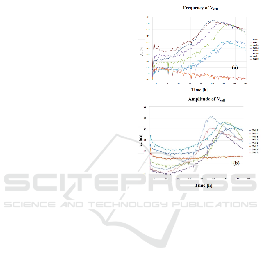
another, and also in time, as consequence of
electrochemical processes in electrode-solution-cell
interfaces. The Fig. 1 shows the oscillation
frequencies measured with our technique (Huertas,
2015) for eight different cell cultures in a growth
curve assay. Each curve shows the oscillation
frequency measured as a function of the time. The
number of cell in the culture increases in time,
depending of the cycle division of the cell line.
Cell-cultures are done with commercial electrodes
(Applied Biophysics), for several number of initial
cells seeded: W1, W3: 2500 cells, W4, W5: 5000
cells; W7, W8: 10000 cells. From these responses, it
can be concluded that:
1) Equal or similar oscillation frequencies were
expected at the beginning of the assays,
because cell density is very low. However, a
wide frequency dispersion can be observed at t
= 0 h, for example.
2) It will be expected a constant frequency
response in cultures with only medium (W2
and W6). However, frequency response
decreases in time from 790 Hz to 760 Hz, after
one week (W2 and W6).
3) Responses of cultures with the same initial
cells (W8-W7, W4-W5, W1-W3) should lead
us to similar oscillation frequencies also. This
is no true: measured frequencies (see W4 and
W5 seeded with 5000 cells, for example) at the
same times, are quite different.
4) The frequency dynamic range of the resulting
frequencies changes between cultures, both for
the same initial and different number of cells.
This experimental performance observed it is also
detected for the amplitude of the oscillations (Fig.
1b). In all cases, measures were done with the same
circuit, so measuring mismatching was not due to
difference on circuit implementation. Considering
these data, the electrical model for electrode-cell-
solution system seems to change from electrode
sample-to-sample, and in time, for the same
electrode sample. This make not possible to consider
a “static” model for the parameter values of the
electrical model defining the performance of this
system, in the sense that these parameters (resistance
and capacitance values linked) will change for each
sample, and also progress in time. It is proposed in
this paper, on that basis of experimental result
analysed, a “dynamic” matching of these
parameters, once each experiment is finished. It is
true that this approach does not allow full prediction
of growth curves, but it will be demonstrated that
errors in measured parameters (frequency and
amplitude of the oscillations) are reduced by the
matching method proposed in the following.
Figure 1: Measured time evolution of the oscillation frequency (a)
and amplitude (b) of voltage signal Vcell. Curves corresponds to
2.500 cells (W1, W3), 5.000 cells (W4, W5) and 10.000 cells
(W7, W8), seeded at t = 0, into separate well pairs. Wells W2 and
W6 contain only medium.
The measurement system is described on section 2
with the sensing principle based on Oscillation
Based Test (OBT) (Huertas, 2015). A method to
solve the system equations is needed to obtain the
oscillation amplitude (a
osc
) and frequency (f
osc
)
(Huertas, 2015, Maldonado, 2016). Also, equations
proposed to match experimental results are derived
to put forward an electrical cell-electrode-solution
model. Section 3 will describe the followed fitting
process. Experimental results are described in
section 4, and finally, conclusions are summarized in
section 5.
2. MATERIALS AND METHODS
2.1 Cell-culture assay
Several experiments were carried out within one
week. The electrodes employed for our tests are
commercial electrodes from Applied Biophysics.
These electrodes contain 8 separated wells with ten
Practical Characterization of Cell-Electrode Electrical Models in Bio-Impedance Assays
101

circular biocompatible gold microelectrodes of 250
m diameter. The biological sample under test is
formed by Chinese hamster ovarian fibroblasts. This
cell line is identified as AA8 (American Type
Culture Collection). This sample is immersed in
McCoy’s medium supplemented with 10 % (v/v)
foetal calf serum; 2mM L-glutamine, 50 μg/ml
streptomycin and 50 U/ml penicilin. The growing
environment is set at 37oC and 5% CO2 in a humid
atmosphere. Different initial number of cells was
planned for our experiments, either 2500, 5000 or
10000.
2.2 Cell-electrode electrical model
The biological sample under test is located on a
two electrode system. The first one acts as a
reference electrode and the second one is the
measurement electrode. Cells are deployed on the
electrodes alongside with medium solution. The
electrical model describing this cell-electrode
interface is presented on Fig 2a. This model has
been explored on the literature in (Borkholder, 1998;
Huang, 2004; Huertas, 2015). The sample is the
connected to the oscillator as shown in Fig 2b, to
build the biological sensor. A start-up signal is
provided to the OBT to provide faster measurements
and assure the optimal oscillation point for the
system thus avoiding nonlinear behaviours of the
electrical model. As it was mentioned in the
previous section, the variation of the BioZ implies a
change on the oscillator values, which is directly
relate to the fill-factor, ff, on the cell culture, thus
allowing us to measure cell population and growth.
Figure 2. (a) Electric model of cell-electrode (BioZ). (b)
Measuring circuit diagram.
The BioZ main electrical-model parameters are C,
the double-layer capacitance arising from the cell
electrode complex and R, the transfer resistance that
represents biological sample resistance. Both
elements are placed in parallel (Huang, 2004;
Huertas, 2015). Fill-factor is presented as the cell
covered area ratio in the electrodes (if there are not
cells, is 0, and it is 1 when electrode is fully
covered).
1
1
2
2
/ (1 )
.(1 )
/
.
R R ff
C C ff
R R ff
C C f
(1)
where C
1
and R
1
account for the empty
microelectrodes contribution to the electrical
response of the biological sample, and C
2
and R
2
depict the electrical response generated by the
electrodes covered by cells. The R
s
models the
resistance which current must overtake to arrive at
reference electrode. Finally, R
gap
represents the
resistance shaped at the gap or interface region
between cell and electrode.
The model fitting process requires further
knowledge on the circuit transfer function. Having
analyzed the electrical model, next step is to define
the transfer functions for the measuring system
(Huertas, 2015; Maldonado 2016; Pérez, 2017). The
analysis is presented below and summarized in eq.
(2).
22
2 1 0
22
()
()
()
o
o
o
o
k s k s k
Vs
Q
Zs
Is
ss
Q
(2)
where,
2 s
kR
(3)
1
1
12
.
2
gap
s
gap
RR
kR
R R R
(4)
12
0
12
()
gap
s
gap
R R R
kR
R R R
(5)
12
0
2
()
gap
gap
R R R
R RC
(6)
12
.
2
gap
o
gap
R RC
Q
R R R
(7)
During the modelling adjustment process, three
challenges were identified:
• Fill-factor: This is the measurement we aim to
find out. This work is part of the process to
obtain a reliable ff measurement out of the a
osc
and f
osc
acquired from the implemented sensor.
To fit the model, we need to use a reliable
reference for ff other than the measurements
itself. This ff reference may be obtained from the
microscopic analysis of the cell cultures under
(a)
(b)
BIODEVICES 2018 - 11th International Conference on Biomedical Electronics and Devices
102

test, but it can be the final solution because the
ultimate goal is getting a sensing robust system
to measure the number of cells without touch the
cell-culture assay until the end of experiment.
• Non-constant value of the BioZ parameters along
ff: The following Bode diagrams acquired from
biological samples under test (Fig. 3) shows that
magnitude at high frequencies can be used to
determine R
s
. However it is important to remark
the differences among different days (cells are
growing, hence increasing ff), which implies also
variations on the R
s
obtained values.
Figure 3: Bode diagram, magnitude and phase, for a single well
during the experiment.
• Each well starts at different values of f
osc
and
a
osc
: Fig. 4 illustrates small differences on each
well in magnitude and phase during the
experiment starting period. Experiment begins at
several hundred Hertz, below 1 kHz, at this
operation point each well has different frequency
and amplitude values. The sample contains eight
wells, each of them contain only either medium
or cells with medium. These one start in an initial
value of f
osc
and a
osc
which does not match with
expected theoretical values for low ff.
Experimental measurements tend to fit the
expected values around 20 hours periods,
corresponding to the cell division cycle.
Figure 4: Bode diagram for each well on the first day.
2.3 Oscillator
Complete closed-loop system (circuit with BioZ)
behaves like an oscillator (Fig 2 (b)). This is due to
the circuit containing a non-linear element, a
comparator in the feedback loop. Non-Linear system
can present oscillations with a constant amplitude
and frequency without external stimulation (limit-
circles). According to describing-function method,
non-linear component of the system can be
linearized like it is presented in equation,
( , )
Y
NA
X
(8)
where N(A, ) is an approximate linear form of
the non-linear element, X is the sine input
amplitude, Y is the amplitude of output fundamental
harmonic component, and is phase difference of
output fundamental harmonic component. In this
case, describing function of comparator is shown in
eq. (9).
4
( ) .( cos( ) sin( ))
ref
hh
osc
V
NA
a
(9)
where V
ref
is the reference voltage for the
comparator and
h
is defined in eq. (10),
sin( )
h
osc
h
a
a
(10)
being h the comparator hysteresis. The shape of
describing-function has been defined. Additionally,
the behaviour of the system is determined by the
characteristic equation (11). If a solution exists for
the given system, with a specific amplitude and
frequency, means that the system is oscillating at
that frequency with given amplitude.
1 ( ) ( ) 0G j N A
(11)
where G(j) is the transfer function for the linear
component of the system, which is the measurement
circuit without the comparator and with BioZ. This is
fulfilled when the following conditions are met:
1. A non-linear component must be part of the
system. In this case non-linear part is the
comparator.
2. Non-linear component does not depend on time.
3. Linear parts behave like a low-pass filter to
guarantee that high frequency harmonics do not
affect non-linear part. The system contains a
band-pass filter, which avoid the input of non-
fundamental harmonic components of the signal
in the comparator.
Practical Characterization of Cell-Electrode Electrical Models in Bio-Impedance Assays
103

4. Non-linearity is symmetrical, so there is not any
DC component in the output signal when input
signal is a sine.
With this method, theoretical a
osc
and f
osc
can be
obtained depending on system parameters. Therefore,
it is necessary to characterize a system model to
compare theoretical and experimental results.
2.4 Sensitivity
To characterize an empirical model it is necessary
to understand how changes in model parameters
affect amplitude and frequency of the oscillation
signal.
2.4.1 Fill-factor
It is important to understand the effects of fill-
factor in the model of BioZ. Considering ff →0, we
can conclude that R
2
→∞ and C
2
→0. Transfer
function for BioZ is presented in eq. (12).
0
( ) ( || )
ff s
Z s R C R
(11)
0
1
.( )
( || )
()
1
s
s
ff
Rs
R R C
Zs
s
RC
(12)
where Z
ff→0
(s) is the impedance of cells for ff→0.
Considering ff→1 we can conclude that R
1
→∞ and
C
1
→0. Transfer function for BioZ is presented in eq.
(14).
1
( ) ( || )
ff s gap
Z s R C R R
(13)
1
()
()
( ) ( )
1
s gap
s gap
ff s gap
R R R
s
RC R R
Z s R R
s
RC
(14)
where Z
ff→1
(s) is the impedance of cells having ff→1.
From equations (13) and (14), the following
statements are deduced. Low ff (experiment
beginning) implies that Rgap does not affect model
behavior. However, high ff implies greater effect on
system model.
2.4.2 Poles and zeros location
It is necessary to identify the position of pole and
zero in transfer function in eq. (14). These are
defined on eq. (15) and eq. (16).
11
( 0)
2 ( | ) 2
z
ss
f ff
C R R CR
(15)
1
( 0)
2
p
f ff
RC
(16)
It is possible now to calculate R
S
and R using eqs.
(17) and (18),
0
0
lim( )( ))
ff s
f
Z s R R
(17)
1
lim( )( ))
ff s
f
Z s R
(18)
by knowing the Bode diagram of the real system
when the experiment starts and finishes. This task
has been performed in three different experiments.
Fig. 4 shows Bode diagrams for well number one
during each day of the experiment. First approach
was to try to fit the model using such Bode diagrams
but it was very difficult to find a suitable fit, as it is
illustrated on Fig. 5.
Firstly, the model of BioZ is far from perfect, so that
it is not possible to get a Bode diagram of the model
similar to experimental Bode diagram. Secondly, it
is difficult to reproduce similar magnitude and phase
at the same frequency in model and experiment.
Thus, it is necessary to find another way to fit the
model. However, it is important to remark that zero
is approximately at 15 kHz in every well and
considered ff. To prove the use of 15 kHz as the zero
value it is compared to another experiment, this is
shown in Fig. 6. This experiment was performed in
one day. Different cells concentrations were put on
all wells, in ascending order, from well one
(medium) until well eight (upper cells
concentrations). Objective of this experiment is to
obtain the Bode diagram of the system for each cell
concentration without medium degradation.
Figure 5: First approach fitting.
BIODEVICES 2018 - 11th International Conference on Biomedical Electronics and Devices
104
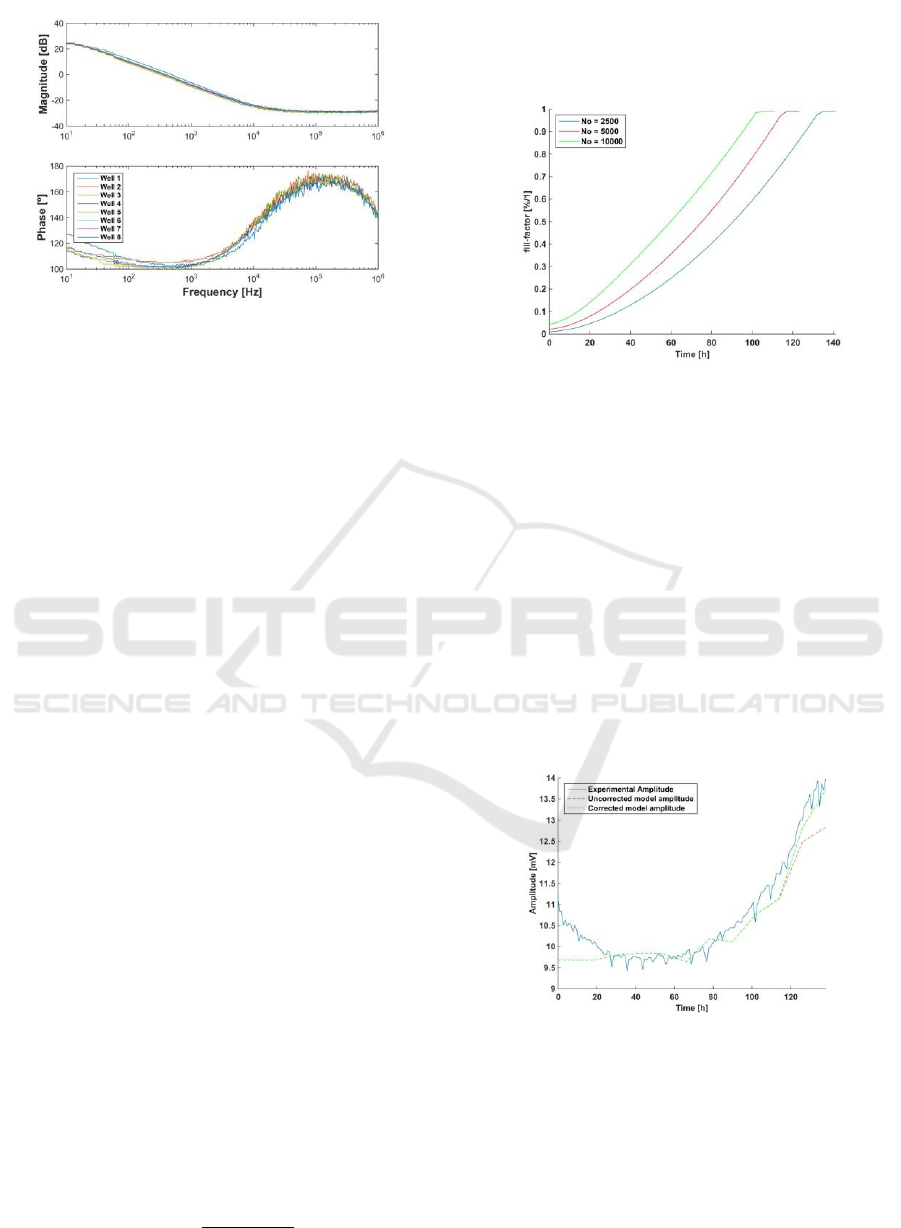
Figure 6: One day experiment
2.4.3: Other parameters
There are some parameters which are yet not
characterized. It is important to consider the effect of
these parameters in frequency and amplitude of the
oscillator. Thank to electric simulator Multisim (and
comparing with theoretical results of Matlab), the
effects can be estimated using parametric sweeping.
Some conclusions are provided below:
• ff→0 (beginning of the experiment):
o Initial frequency can be selected only with
position of the pole fp.
o Initial amplitude can be selected using R
s
and f
p
.
The R
s
effect is significantly higher.
• ff→1 (end of the experiment). Frequency can be
selected using R
gap
, however it is important to
remark that R
gap
affect final amplitude as well.
It is possible to characterize the model parameters
using this conclusions and eqs. (15) and (16).
2.5 Estimation of ff
During first experiment, which Bode diagrams
were measured, wells were also photographed to
estimate ff once a day until the end of the
experiment. However, estimation of ff using photos
was not accurate enough. On the following, a math
temporal evolution estimation method for ff is
presented.
Considering the area of the well is A
w
=0.8 cm
2
,
approximate radio of cells is r
cell
= 10 μm
2
. Knowing
the number of cells at the beginning of experiment
as N
o
and the division time of cells as t
r
= 18 hours,
it is possible to define a growth curve for (ff) in time.
( ) 2
k
o
N k N
(19)
2
()
cell
k
w
N k r
ff
A
(20)
Using eqs. (19) and (20), it is possible to calculate
the number of cells and ff at a given moment, k, as is
shown in Fig. 7.
Figure 7: Estimated evolution of ff with No = 2.500, 5.000 and
10.000 cells.
3. Fitting model
There is enough information to fit the experiment
model. Keeping in mind that f
z
= 15 kHz, the
algorithm to obtain the model:
Step 1: Select f
p
using experiment initial frequency.
Step 2: Select R
s
using experiment initial amplitude.
Step 3: Select R
gap
using experiment final frequency.
Following this three steps, it is possible to fit a
model which behaves similar to the experimental
results. Even so, there is an amplitude error that
increases with ff, observed in Fig. 8.
Figure 8: Comparison between experimental amplitude,
uncorrected and corrected model amplitudes.
To solve this problem, first approach is to use the
work presented in (Huang, 2004), but performing an
alternative correction of R
s
with ff. Moreover, it is
decided that parameter R
s
, which is calculated for ff
→0, is an initial value of R
s
, named R
si
. R
s
grows
with ff during the whole experiment. R
s
must match
Practical Characterization of Cell-Electrode Electrical Models in Bio-Impedance Assays
105
the amplitude in ff → 1. This is represented on eq.
(21).
( ) . ( )
n
s si s
R k R R ff k
(21)
where R
si
is the initial value for R
s
, R
s
is the range
of R
s
from ff = 0 to ff = 1, and n decided the growth
rate of R
s
until the maximum value (n=4 in this
case). The eq. (21), represents R
s
variation, allowing
R
s
to reach its final value when well is full (R
s
(ff
→1) = R
si
+R
s
). Finally, it is necessary to complete
the fitting model selecting R
s
.
Step 4: Select R
s
using experiment final amplitude.
The Fig. 7 shows the effect of the evolution of R
s
,
with good agreement for amplitude estimation.
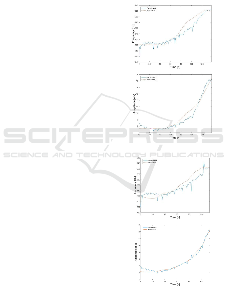
4. RESULTS
This section presents the results of the fitting
method proposed before. Results are shown from
Figures 9 to 11 (each figure shows one well with
cells), and start from three different values of initial
number of cells: 2500, 5000 and 10.000 cells. For
each initial number of seeded cells, the time
evolution of the ff is calculated according to eq. (20),
and then, electrical simulations are performed in
Multisim, considering the proposed parameters
evaluated for the electrical model. The oscillation
parameters, f
osc
and a
osc
, are measured and compared
with the experimental ones.
In all cases, the amplitude and frequency errors
are reduced, being possible to make the cell number
estimation, at every time of the experiment. Errors
observed at amplitudes are lower than frequencies.
One of the main problems to fit the models of each
well of the experiments is the small range of a
osc
and
f
osc
found on the available data. Using this method,
theoretical results are similar to experimental results.
5. CONCLUSIONS
It has been presented a fitting procedure to
assign values to proposed parameters of the
electrical-model in cell cultures assays. The proposal
is useful in ECIS experiments to define the number
of cells in a culture, giving a general solution, not
only for cell monolayer configurations. For several
initial
values of cell seeded, results show that fitting
models
provide low error estimations for ff values.
Thanks
to ff estimation and R
s
modification, it is
possible
to fit a model for each well knowing only
a
osc
y
f
osc
values at beginning and end of the
experiment.
A Matlab script has been developed to do
this
work automatically when experiment ends,
either
using theoretical equations of the system or
using the
software Multisim software to execute
electrical simulations.
Figure 9: Comparison of frequencies and amplitudes between
model and experiment for No = 2500 cells.
BIODEVICES 2018 - 11th International Conference on Biomedical Electronics and Devices
106
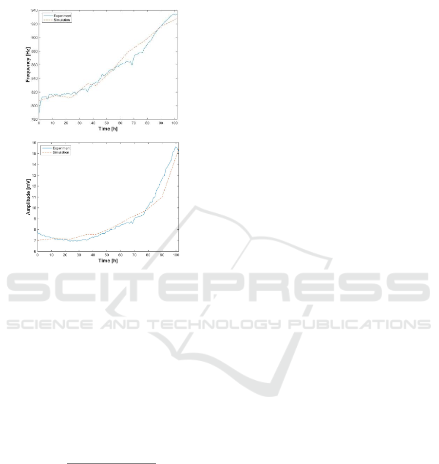
Figure 10: Comparison of frequencies and amplitudes between
model and experiment for N
o
= 5.000 cells.
Figure 11: Comparison of frequencies between model and
experiment for N
o
= 10.000 cells.
ACKNOWLEDGMENT
This work was supported in part by the Spanish
founded Project: Integrated Microsystems for cell
culture test (TEC2013-46242-C3-1-P), co-financed
with FEDER program.
REFERENCES
Abdolahad, M., Shashaani, H., Janmaleki, M., Mohajerzadeh, S.,
2014. “Silicon nano grass based impedance biosensor for
label free detection of rare metastatic cells among primary
cancerous colon cells, suitable for more accurate cancer
staging,”. Biosensors and Bioelectronics, 59, 151-159.
Applied Biophysics (http://www.biophysics.com/).
Borkholder, D. A., 1998. ”Cell based biosensors using
microelectrode”. Ph D. Thesis.
Daza, P., Olmo, A., Cañete, D., Yúfera, A., 2013. “Monitoring
living cell assays with bio-impedance sensors”. Sensors and
Actuators B: Chemical. 176, 605-610.
Dibao-Dina, A., Follet, J., Ibrahim. M., Vlandas, A., Senez, V.,
2015.“Electrical impedances sensor for quantitative
monitoring of infection processes on HCT-8 cells by the
water borne parasite Cryptosporidium,” at Biosensors and
Bioelectronics, 66, 69-76.
Grimnes, S. and Martinsen, O., 2008. Bio-impedance and
Bioelectricity Basics. 2nd edition. Academic Press, Elsevier.
Giaever, I. and Keese, C. R., 1986. “Use of Electric Fields to
Monitor the Dynamical Aspect of Cell Behaviour in Tissue
Cultures”. IEEE Transactions on Biomedical Engineering,
vol. BME-33, nº 2, 242-247.
Huang, X., Nguyen, D., Greve, D. W. And Domach, M. M., 2004.
”Simulation of Microelectrode Impedance Changes Due to
Cell Growth” IEEE Sensors Journal, vol. 4, n
o
. 5.
Huertas, G., Maldonado-Jacobi, A., Yúfera, A., Rueda, Huertas,
J- L., 2015. “The Bio-Oscillator: A Circuit for Cell-Culture
Assays,” IEEE Trans on CAS-II. 62, 164-168.
Khalil, S. F., Mohktar, M. S. and Ibrahim, F., 2014. ”The Theory
and Fundamentals of Bioimpedance Analysis in Clinical
Status Monitoring and Diagnosis of Diseases” Sensors,
14(6): 10895 – 10928.
Lei, K. F., 2014. ”Review on Impedance Detection of Cellular
Responses in Micro/Nano Environment” Micromachines.
Lourenco, F., Ledoa, C. A., Laranjinhaa, J., Gerhardtc, G. A.,
Barbosa, R. M., 2016. “Microelectrode array biosensor for
high-resolution measurements of extracellular glucose in the
brain,”. Sensors and Actuators B: Chemical. 237, 298-307.
Lu, Y-Y., Huang, J-J. and Cheng, K-S., 2009. ”The design of
electrode-array for monitoring the cellular bioimpedance”
Industrial Electronics and Applications.
Maldonado, A., Huertas, G., Rueda, A., Huertas, J. L., Pérez, P.
and Yúfera, A., 2016. ”Cell-culture measurements using
voltage oscillations” IEEE 7
th
Latin American Symposium
on CAS (LASCAS).
Pérez, P., Maldonado-Jacobi, A., López, A., Martínez, C., Olmo,
A., Huertas, G. and Yúfera, A., 2017. “Remote Sensing of
Cell Culture Assays. Cell Culture,” Chap 4: New Insights
in Cell Culture Technology. 135-155. InTech Europe.
Pradham, R., Mandal, M., Mitra, A., Das, S., 2014. “Monitoring
cellular activities of cancer cells using impedance sensing
devices”. Sensors and Actuator B: Chemical, 193, 478-483.
Reitinger, S., Wissenwasser. J., Kapferera, W., Heer, R.,
Lepperdinger, G., 2012. “Electric impedance sensing in cell
substrates for rapid and selective multipotential
differentiation capacity monitoring of human mesenchymal
stem cells,”. Biosensors and Bioelectronics, 34, 63-69.
Practical Characterization of Cell-Electrode Electrical Models in Bio-Impedance Assays
107
