Traffic Signs Recognition and Classification based on Deep Feature
Learning
Yan Lai, Nanxin Wang, Yusi Yang and Lan Lin
School of Electronics and Information Engineering, Tongji University, Shanghai, China
Keywords:
Traffic Signs Recognition, Convolutional Neural Network, YCbCr Color Space, Support Vector Machine.
Abstract:
Traffic signs recognition and classification play an important role in the unmanned automatic driving. Various
methods were proposed in the past years to deal wi th this problem, yet the performance of these algorithms
still needs t o be improved to meet the requirements in real applications. In this paper, a novel tr affic signs
recognition and classification method is presented based on Convolutional Neural Network and Support Vec-
tor Machine (CNN-SVM). In this method, the YCbCr color space is introduced in CNN to divide the color
channels for feature extraction. A SVM classifier is used for classification based on the extracted features.
The experiments are conducted on a real world data set with images and videos captured from ordinary car
driving. The experimental results show that compared with the state-of-the-art methods, our method achieves
the best performance on traffic signs recognition and classification, with a highest 98.6 % accuracy rate.
1 INTRODUCTION
Nowadays, unmanned automatic driving technolog y
(Sezer et al., 2011) has attracted increa sin g atten tions
from researches and industry communities. The traf -
fic signs recognition and classification play an impor-
tant role in this field. A lots of resear ch efforts have
been d evoted to dealing with the problem. However,
many factors, such as insufficient illumination, par-
tial occlusion and serious deformation, make traffic
detection a challenging problem.
Feature extraction in traditional traffic signs re-
cognition is based on ha nd-crafted methods, such as
Scale-Invariant Feature Transform (SIFT) (Nassu and
Ukai, 2010), Histogram of Oriented Gradient (HOG)
(Creusen et al., 2010) and Speeded-Up Robust Featu-
res (SURF) (Duan and Viktor, 2015). With the rise of
neural network theory, the applicatio n in recog nition
has also increased, e.g., the Semantic Segmentation-
Aware CNN Model (Gidaris and Komodakis, 2015),
showing a better feature-learning capabilities.
Even though traffic signs detection and classifica-
tion h a d been developed fo r a long time, a complete
data set was inadequate until the launch of the Ger-
man Traffic Signs Recognition Ben chmark (G TSRB)
(Stallkamp et al. , 2012) and Detection Benchmark
(GTSDB) (Houben et al., 2014). Various methods
have been making progress in these two tasks, such
as the DP-KELM method (Zeng et al., 2017). Howe-
(a) Warning (b) Prohibition (c) Mandatory
Figure 1: Three Main Categories of Traffic Signs in China.
Warning signs (mostly yellow triangles with a black boun-
dary), P r ohibition signs (mostly white surrounded by a red
circle) and Mandatory signs (mostly blue circles with white
information).
ver, the GTSDB cannot adapt very well in real world
tasks, due to the small size of the training data. Af -
ter that, a b enchmark named Tsinghua-Tencent 100K
(Zhu et a l., 2 016) has been proposed a long with th e
end-to-end CNNs method, which shows a good p er-
formance of detection and classification of tiny traffic
signs. However, the processing speed is still slow.
In this p aper, three main traffic signs categories,
i.e., warning signs, prohibition signs and mandatory
signs (shown in Figure 1), are covered for experi-
ments. Specifically, in our video-based CNN-SVM
recogn ition framework, b y introducing the YCbCr co-
lor space (Basilio et al., 2011), we firstly divide the
color channels, secondly employ CNN deep network
for deep featu re extraction and then ado pt SVM for
classification. The experiments are conducted on a
real world data set, based on which, a sy nthetically
compariso n illustrates the superiority of our model.
622
Lai, Y., Wang, N., Yang, Y. and Lin, L.
Traffic Signs Recognition and Classification based on Deep Feature Learning.
DOI: 10.5220/0006718806220629
In Proceedings of the 7th International Conference on Pattern Recognition Applications and Methods (ICPRAM 2018), pages 622-629
ISBN: 978-989-758-276-9
Copyright © 2018 by SCITEPRESS – Science and Technology Publications, Lda. All rights reserved

The re st of the paper is organ ized as fo llows:
Section 2 discusses the relate d work. The frame-
work and experimental data are shown in Section 3,
while the introduction of the YCbCr-based network
is presented in Sectio n 4. The parameters adjustment
and image preprocessing in CNN-SVM are done in
Section 5. Finally, we give experimental results in
Section 6 and conclusions in Sec tion 7.
2 RELATE WORK
To solve the target rec ognition problem, most of the
previous works use hand-crafted feature extracting
methods mentioned in Section 1. Those conventio-
nal feature extraction methods, over-reliant on the de-
signer’s experience, meet some restriction in featur e
expression. On the co ntrary, the deep network mo-
del based on CNN is more powerful in feature ex-
pression. CNN method, which possessing th e c ha-
racteristics of rota tion, translation and scaling inva-
riance, is able to realize weight sharin g th rough lo-
cal receptive fields. It’s widely used in the sub-area
of target recognition, e.g., image classification (Kri-
zhevsky et a l., 2012) ( Schmidhuber, 2012), face re-
cognition (Sun et al., 2014) (Li et al., 2015) and pe-
destrian detection (Ouyang and Wang, 2014) (Zeng
et al., 2013) . Afterwards, various CNN-based mo-
dels have been proposed, such as AlexNet (Krizhe-
vsky et al., 2012), VGG (Simonyan and Z isserman,
2014) , GoogleNet (Szegedy et al., 2015 ), ResNet (He
et al., 2016) and so on. The VGG network mo del has
been widely used and improved by researchers thanks
to its multi-layer construction and excellent perfor-
mance on the most representative data set in target re-
cognition field which na med ImageNet (Krizh evsky
et al., 2012). Based on this, some famous network
models, e.g., the R-CNN series (Girshick, 2015) (Ren
et al., 2017), YOLO (Redmon et al., 2016), SSD (Liu
et al., 2016) , R-FCN (Dai et al., 201 6), appears in
succession.
3 FRAMEWORK AND
EXPERIMENTAL DATA
3.1 Framework of CNN-SVM Method
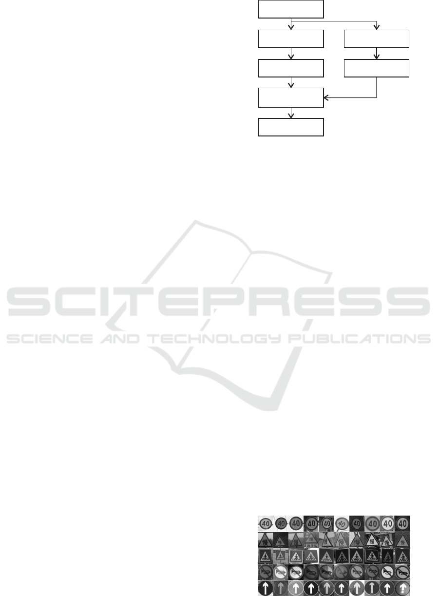
Figure 2 shows a process diagram of the working pro-
cedures of CNN-SVM. The CNN-SVM method can
be concluded as the following six steps:
• Training images and testing street-view images
Raw I mages
Training Images
Testing Im a ges
Feature Extraction
Preprocessing
Classification
Result
ROIs
Figure 2: Framework of Traffic Signs Recognition.
are collected, and then the tra ining images are la-
beled and transformed in YCbCr color space.
• Visual features of these training images are ex-
tracted in CNN.
• A SVM classifier is used to classify the train ing
images based on the extracted feature s.
• Testing street-view images are sent to preproces-
sing progress, including homomorphic filter, mor-
phological treatment and area threshold segmen-
tation.
• Region of In te rest (ROIs) in street view are acqui-
red and delivered to CNN-SVM mod el.
• Detection and classification resu lts are obtaine d.
3.2 Experimental Data
Eight kinds of signs, individually from the warning
signs, prohibition signs and mandatory signs, are ta-
ken into consideration in o ur research. The trai-
ning imag es mainly co nsists of mobile phone sho ot-
ings, GTSDB and Baidu exploration. These image s,
through some transformation like rotating and affine
transformations, reach a total number of 1000. Each
image is unified with the size of 48× 48. Then, th e se
images are labeled and composed as a training data set
which is shown in Fig ure 3. The testing street-view
images comes from 4 videos, wh ic h are captured by
PIKE F-100 FireWire camera. Each frame size of the
videos is 1920×1080.
Figure 3: Traffic Signs Training Data Set.
Traffic Signs Recognition and Classification based on Deep Feature Learning
623

L
Img
·
f
x
b
x
∑
C
x
∑
X
w
x+1
b
x+1
S
x+1
Figure 4: The Diagram of Convolution Progress. An input
sample with the size of 48×48 is convoluted with a 5×5
convolutional kernel. Then, six 44×44 feature maps are ge-
nerated. Each neuron in the feature map is connected with
5×5 convex kernel. After the summation of each group of
pixels in the feature map, the weight and offset are added.
After taking activate function, the neurons in the next layer
are automatically acquired. Naturally, the next volume can
be obtained by continuous translation and traverse opera-
tion.
4 CONVOLUTIONAL NEURAL
NETWORK TRAINING BASED
ON YCBC R COLOR SPACE
4.1 Convolutional Neural Network
Our basic model follows the classic LeNet-5 network,
which consists of three co nvolutional layers (C
1
, C
3
and C
5
) and two sub-sampling layers (S
2
and S
4
). The
input of each layer represents a small group of local
units from the upper layer. Each convolution layer
contains multiple convolution kern e ls. These convo-
lution kern e ls are ab le to scan the image features via
different expressions, based on this, we can acquir e
various feature maps in different locations. T he sub-
sampling layer, following the convolution layer, is
mainly used to reduce the reso lution of the feature
map, to extra ct the existing image features and to de-
termine the features’ relative location.
4.2 CNN Training
The training of the layer-concatena ted CNN in c ludes
4 main parts, i.e., forward propagation, error calcula-
tion, back p ropagatio n and weights adjustment. The
forward propagation represents a progr ess of infor-
mation delivery from the input layer to the output
layer. Since initialization of the weightin g parame-
ters is random, the results obtained by forward propa-
gation tend to be deviated. To modify this deviation,
error estimation and parameters adjustment are inclu-
ded between each forward and backward propagation.
More specifically, it runs with the following pro c edu-
res:
• Extract a sample from the training data set and
send it into the training network.
• Each layer ’s output, generated b y the activation
function, are continuously led into the next hidden
layer till the output layer.
• Calculate the deviation matrix of the ou tput.
• Conduct a layer-by-layer reverse calculation ac-
cording to gradient descent algorithm.
• Acquire the updated weight and gradient values.
• Repeat the forward propagation to start the next
iteration.
4.3 YCbCr Color Space for CNN’s
Feature Extraction
The pr evious traffic signs recognition and classifi-
cation methods usually take CNN training in RGB
space. In that sp ace, the color information and the lu-
minance information are mixed among channe ls, ge-
nerating the variance of the extracted features. No-
netheless, the color distribution in RGB space is not
unifor m. Some subtle changes in color are captured
difficultly.
YCbCr color space is mainly used for continuous
image processing in the video. We can calculate each
component by the transform formula shown a s:
Y = 0.299R + 0.587G + 0.114B (1)
Cb = 0.564(B − Y) (2)
Cr = 0.713(R −Y), (3)
where Y is luminance component, Cb represents the
blue chrominanc e compon e nt and Cr denotes the r e d
chrominance component.
In o rder to choose a better color sp ace for fea -
ture extraction, we conduct an error evaluation amon g
three typical color space, i.e., Grayscale, RGB and
YCbCr. To do this, we send the tra ining data set for
CNN tra ining. Taking the b
n
as the number of wro ng
samples in each batch training , the n as the numbe r
of batch training time, the S as the ba tc h size. We
are able to calculate the training error in each batch
training which r epresented by E
n
:
E
n
=
b
n
S
(4)
The results of different training errors shown as Table
1, we c an find that the corresponding result o f YCbCr
space is better than the othe rs.
Table 1: Training Error in Different Color Spaces.
Color Space Training Error
Grayscale 0.138
RGB 0.105
YCbCr 0.073
ICPRAM 2018 - 7th International Conference on Pattern Recognition Applications and Methods
624

5 PARAMETERS ADJUSTMENT
BASED ON CNN-SVM
In this section, we will take training data set and tes-
ting street-view images to conduct parameters adjust-
ment and image preprocessing in training and testing
progress respectively. The goal of parameters adju s-
tment is to increase training accu racy and to shorte n
the training time in the tr aining parts. While in the
testing progress, the image preprocessing operation is
mainly used to eliminate the negative impacts, e. g.,
insufficient illumination and similar background, so
as to acquire ROIs precisely.
5.1 Parameters A djustment for
Training
In the training p art, some parameters, e.g ., kernel
size, iteration numbers and the connec ting methods
between convolutional layer and sub- sampling layer,
greatly impact on trainin g accuracy and speed. Thus
some experiments are carried out based on the trai-
ning data set for choosin g the best parameters.
5.1.1 Kernel Size
In terms of kernel size, a comparison exp e riment is
condu c te d both in the 2-hidden-layer network and the
4-hidden-layer network. In the 2-hidden-layer net-
work, an input layer, a convolutional layer, a sub-
sampling layer and an output layer are included.
While in the 4-hidden-layer network, ther e exists one
more convolution layer and sub-sampling layer. In
addition, the kernel sizes of the convolution layer se-
lected for the former a re 9×9 and 5×5, yet 7×7 and
5×5 for the late r. This comparison proves that a larger
correspo nding kernel size ref e rs to less convolution
layers, contributing to a higher train ing speed and less
parameters. However, the over large size will cause
the loss of local features.
Table 2: Training Time of Different Kernel Sizes.
Hidden Layers 2 2 4 4
Kernel Size 9×9 5×5 7×7 5×5
Training Time 377s 260s 481s 325s
5.1.2 Connecting Methods
The connection modes between the sub-sampling
layer and the convolution layer include two methods,
i.e., the fully connected method and the non-fully con-
nected method. In order to connect more features,
sub-samplin g layer S
2
and convolution layer C
3
is
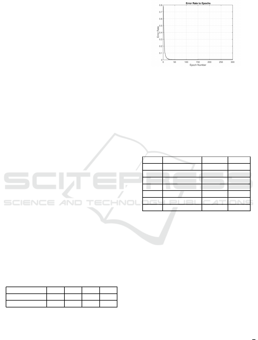
Figure 5: Training Error Rate with 300 Epochs.
fully connected. In this case, there are a total num-
ber of 16×(6×5×5 + 1) = 2, 416 training parameters
accordin g to Ta ble 3. Thus, this connection method
will lead to an increasing of computational cost. In
the deeper layers, we can take the non-fully connected
method like the connection between S
4
and C
5
to re-
duce the information re dundancy. Taking this met-
hod, we can effectively reduce the training parameters
which access to less but more useful features.
Table 3: CNN Constructing Parameters.
Layer Type Neurons Kernel
0 Input 48×48
1 Convolutional 44×44 5×5
2 Subsampling 22×22 2×2
3 Convolutional 18×18 5×5
4 Subsampling 9×9 2×2
5 Convolutional 5×5 5×5
6 Fully 1×600
5.1.3 Iteration Numbers
Theoretically, a higher iteration number, means a
more thorough process. We are able to get more fe-
atures fro m eac h iteration. However, the redund ant
iteration number will lead to an increase of training
error, if noise or the non-representative features in the
photos are fitted. Thus, a test with several iter ation
numbers is conducted. We firstly load the training
data set for the test and choose the iteration number s
of 300. As shown in the Figure 5, we can find th at the
error rate of training process exp eriences a slig ht in-
crease after it converging to a very low rate with 150
epochs, which may ascrib e to the introduce of non-
representative features.
Going deeply, we can load the training da ta set,
randomly select the number of T as training samples,
the rest are testing samples for validation. The to-
tal batch training time can be represented by N =
T
S
.
Based on the Formula 4, the recognition accuracies
which is de fined as A can be calculated by the For-
mula:
Traffic Signs Recognition and Classification based on Deep Feature Learning
625

A = (1 −
N
∑
n=1
(E
n
)
N
) × 100% (5)
We are able to test th e recognition accuracies with
the pa rameters T =840 and S=60, the results of CNN
accuracies with different iteration numbers are shown
in Ta ble 4, in which th e I represent Iterations and A
means Accuracy. Clearly, th e 150-epoch-iteration is
verified to be the best.
Table 4: C N N Accuracies of Different Iterations.
I (epochs) 100 150 350 500
A (%) 97.27 98.18 94.4 92.73
Briefly, the experim e ntal parameters can be con-
cluded in Table 5.
Table 5: CNN E xperimental Parameters.
Kernel Size Batch Size I (epochs)
5×5 / 2×2 60 150
In orde r to optimize the classifying performance,
we have trained the SVM classifier by libsvm package
(Suralkar et al., 2012) (Chang and Lin, 2011) after
removing fully co nnected layer. The output vector
of the last la yer in CNN is regarded as the input of
the SVM. We are able to expand the normal classi-
fier to solve the multi-classify problem, with training
and connecting
k×(k− 1)
2
normal classifier as the con-
struction of a bina ry tree, in which k represents the
number of classes. Kernel function is a key factor
in constructing the SVM classifier. Th e re are several
kernel functions provided for us to select, e .g., RBF,
Linear and Gaussian Kernel, with different parame-
ters and o utcomes. Ta king 100% and 50% training
data set as the experimental samples, we are able to
condu c t an experiment to c hoose th e most suitable
kernel function as Table 6. The overall training time
and trainin g accuracy are two factors to evaluate the
performance of different functions.
From the point of training accuracy, the RBF ker-
nel outperforms the Linear kernel. As the parameter
number of RBF is more than Linear kernel, it will take
times to fin d a better result. Based on large number
of parameters, the training speed of RBF is obviously
slower than the Linear kernel. Thus, th e Linear kernel
can be a more suitable choice for our model. In addi-
tion, the Table 6 also illustrate tha t the SVM method
is robust when the training data set is in a small scale.
Because our data set only contains 1000 image s, the
50% of them still show good performance.
Table 6: The Performance of Different Kernel S izes.
Training Data Kernel Accuracy Time
100% RBF 98.81% 507s
100% Linear 98.6% 371s
50% RBF 96.41% 285s
50% Linear 96.1% 122s
(a) Original (b) Homomorphic (c) Gamma
Figure 6: Comparison between Homomorphic Fi ltering and
Gamma Correction.
5.2 Preprocessing for Testing
Before testing progress, we have to take some image
preprocessing o perations in street-view images to eli-
minate the effect of insufficient illumination, partial
occlusion and serious deformation . The main prepro-
cessing operations include image enhancement and
image segmentation.
Firstly, we need to deal with the images under a
poor illuminatio n. A typical method is the homo-
morphic filter method (Cai et al., 2011), which uses a
suitable homomorphic filter function H(u, v). In this
method, the coefficients are H
l
< 1 and H
h
> 1, the
function H(u, v) would decrease. Therefore, we are
able to enhance the images by reducing the low fre-
quency and increasing the high frequency. Another
way is gamma correc tion (Huang et al., 2013), which
compen sates the deficiency in dim light. The Figure
6 shows a comparison of the homomorphic filtering
as Figure 6 (b) and gamma correction as Fig ure 6(c).
Clearly, the former performs better, as the colo r of
the testing image has a certain distortion after gamma
correction.
In addition , the ima ges with normal light will not
be sent to the filtering process directly. To jud ge the
predicab le images, we can introduce the YCbCr co lor
space, as the Y component represents the illumina-
tion factor. We are able to select the thresholds by
drawing the pixel distribution in histogram and co un-
ting the pixel numbers (a), in images with extremely
light. After taking the experiments, the threshold can
be determined by Y∈[200,234] and a < 53901.
Secondly, we need to take morphological treat-
ment before segmentation to eliminate disco ntinuous
tiny areas. H owever, some obstacles in the street view
have not been removed to ta lly, for instance, the non-
signs areas which are similar with th e signs areas.
Thus, we define the size and proportion of the traf-
fic signs by experimental results. In addition, the one
ICPRAM 2018 - 7th International Conference on Pattern Recognition Applications and Methods
626

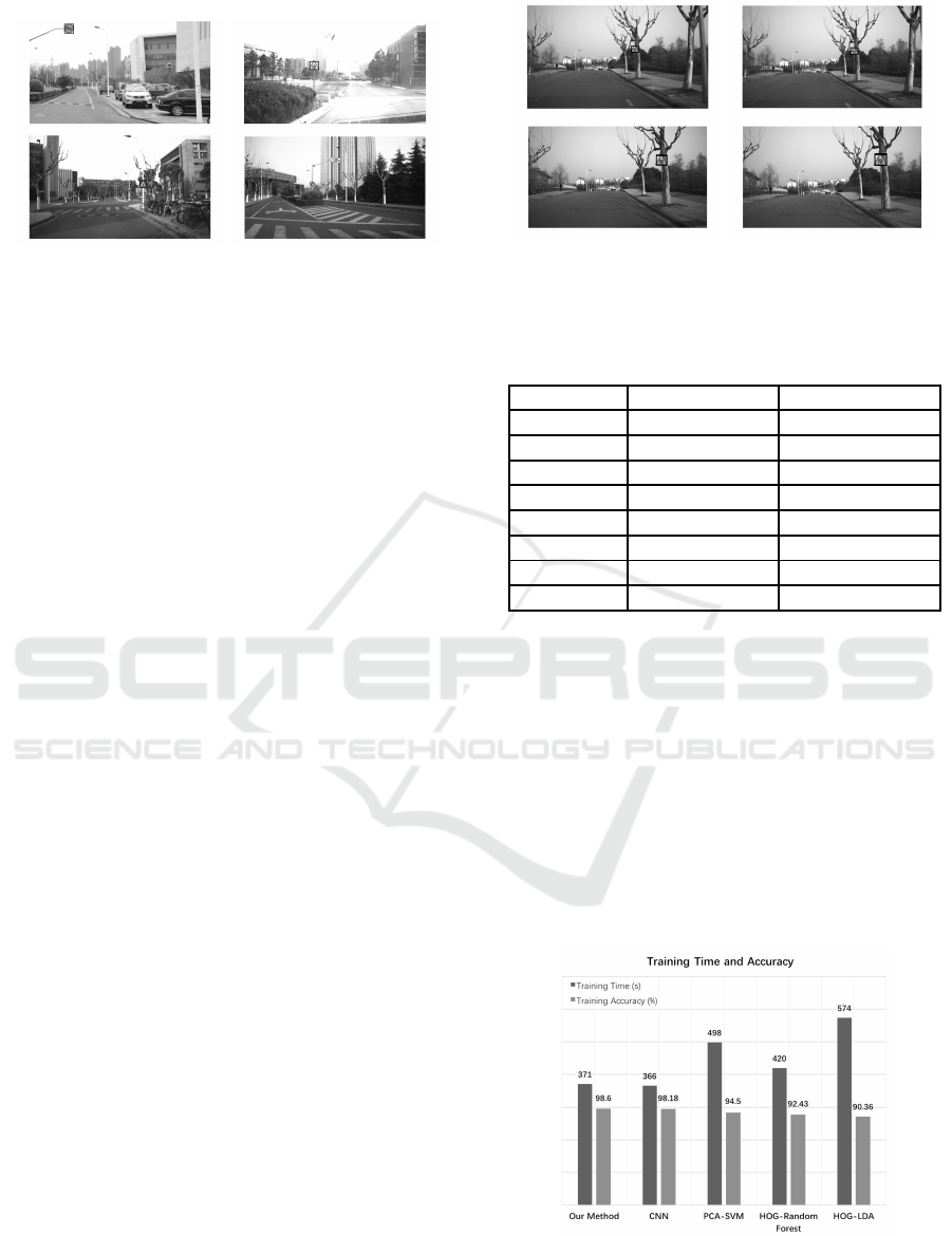
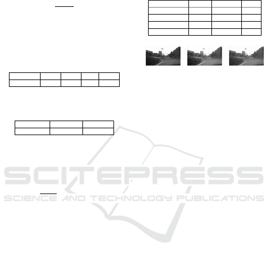
Figure 7: ROIs in Different Scenarios.
third part in the bottom image, where we set the pixel
value to zero, would not co ntain any signs. Thu s, the
non-signs area can be re moved.
Finally, the ROIs can b e selected by a bounding
box with fixed size and proportion in the whole street-
view image as shown in Figure 7. Among these re-
sults, we can find that the most of traffic signs are
successfully recognized while some are ignored or
double reco gnized.
6 ANALYSIS OF EXPERIMENTAL
RESULTS
In this paper, both trainin g and testing were done on
a Linux PC with an Intel i7-6900k CPU an d NVIDIA
GTX 1080 Ti GPU. The collected training data set is
loaded and trained in our network. From the training
data set, we randomly select 840 images as training
samples, the rest as testing samples for cross valida-
tion.
6.1 CNN-SVM Recognition and
Classification Results
The CNN is able to detect an d classify the targets,
via extracting the tra ining samples’ features. Then,
SVM contribute to a better result in classification.
With a number of parameter adjustments, the CNN is
successfully trained with 98.18 % accuracy rate, while
the CNN-SVM’s accuracy reach es 98.6 %. Even
though the growth of accuracy is slight, the training
time is very near from each other, with 366s and 3 71s
respectively.
In addition, we take the mean shift method (Co-
maniciu and Meer, 2002) to track the traffic signs in a
short video as Figure 8. The figure sh ows that th e ca-
pabilities of this fr amework in detecting the tiny traf-
fic signs which take a small area as 0.2 %−0.4 % of
the whole image. The results of the recognition and
classification of 8-classes traffic sign s are shown in
Ta ble 7.
Figure 8: Tracking in Video by Mean Shift. From the upper
left to the lower right sub-images represent the 1st, 3rd, 5th
and 8th frame respectively.
Table 7: The Results of the Recognition and Classification
of 8-classes Traffic Signs.
Classes Total Numbers CNNs-SVM(%)
Limit 30 109 97.34
Limit 40 123 98.32
Limit 50 141 98.7
Slow 136 98.9
Crossroads 134 98.56
No tooting 153 99.4 3
Right 138 98.4 6
Straihgt 66 96.6
6.2 Comparison with State-of-the-Art
Methods
The Figure 9 illustrates the co mparison results with
other state-of-the-art method s. It shows that our
CNN-SVM method is able to achieve a highe r accu-
racy (98.6%) than the others, e.g., HOG-LDA (Stal-
lkamp et al., 2012), HOG-Random Forest (Zaklouta
et al., 2011) a nd PCA-SVM (Chan et al., 2015). Furt-
hermore, the training time of our method ( around
371s) is the fastest, wh ic h nearly twice as fast as the
HOG-LDA.
Figure 9: Comparison with State-of-the-Art Methods.
Traffic Signs Recognition and Classification based on Deep Feature Learning
627

7 CONCLUSIONS
In this paper, a recognition and classification method
based on CNN-SVM has been proposed. In the trai-
ning process, the deep image features are extracted
by CNN in the YCbCr color space. SVM is con-
nected with the last layer of CNN fo r fur ther classi-
fication, which contributes to a better trainin g results.
On the other hand, some images preprocessing pro-
cedures are conducted in the testing p rocess, in or-
der to eliminate those negative impacts, e.g., insuffi-
cient illumination, pa rtial occlusion and serious de-
formation. Experiment-based comparison with oth e r
state-of-the-art methods verify that ou r model is su-
perior than the others both in training accuracy and
speed. Furthermore, we found that some traffic signs
are miss-recognize d when we apply this method in the
unmanned ground vehicle. In ne ar future, we p lan to
expand our data set by seeking out more images of
traffic signs, especially the images a t night. Then, we
will accelerate the speed by optimizing the algorithm
for real- time application in vehicles.
ACKNOWLEDGEM EN TS
This work was supported b y the Natio nal Natu-
ral Science Found ation of China (NSFC), G rant
No.61373106. The authors gratefully acknowledge
everyone who helped in the work. Correspond ing
author: Lan Lin.
REFERENCES
Basilio, J. A. M., Torres, G. A., Rez, G. S., nchez, Medina,
L. K. T., Meana, H ., and Ctor, M. P. (2011). Explicit
image detection using ycbcr space color model as skin
detection. In American Conference on Applied Mat-
hematics and the Wseas International Conference on
Computer Engineering and Applications, pages 123–
128.
Cai, W., Liu, Y., Li, M., Cheng, L. , and Zhang, C. (2011).
A self-adaptive homomorphic filter method for re-
moving thin cloud. In International Conference on
Geoinformatics, pages 1–4.
Chan, T. H ., Jia, K., Gao, S., Lu, J., Zeng, Z., and Ma, Y.
(2015). Pcanet: A simple deep learning baseline for
image classification? IEEE Transactions on Image
Processing A Publication of the IEEE Signal Proces-
sing Society, 24(12):5017–5032.
Chang, C. C. and Lin, C. J. (2011). LIBSVM: A library for
support vector machines. ACM.
Comaniciu, D. and Meer, P. (2002). Mean shift: A robust
approach toward feature space analysis. IEEE Tran-
sactions on Pattern Analysis & Machine Intelligence,
24(5):603–619.
Creusen, I . M., Wijnhoven, R. G. J., Herbschleb, E., and
With, P. H. N. D. (2010). Color exploitation in hog-
based traffic sign detection. I n IEEE International
Conference on Image Processing, pages 2669–2672.
Dai, J., Li, Y., He, K. , and Sun, J. (2016). R-fcn: O bject de-
tection via region-based fully convolutional networks.
Duan, J. and Viktor, M. (2015). Real time road edges de-
tection and r oad signs recognition. In International
Conference on Control, Automation and Information
Sciences, pages 107–112.
Gidaris, S. and Komodakis, N. (2015). Object detection via
a multi-region and semantic segmentation-aware cnn
model. In IEEE International Conference on Compu-
ter Vision, pages 1134–1142.
Girshick, R. (2015). Fast r-cnn. In IEEE International Con-
ference on Computer Vision, pages 1440–1448.
He, K., Zhang, X., Ren, S., and Sun, J. (2016). Deep resi-
dual learning for image recognition. Computer Vision
and Pattern Recognition, pages 770–778.
Houben, S., Stallkamp, J., Salmen, J., Schlipsing, M., and
Igel, C. (2014). Detection of traffic signs in r eal-
world images: The german traffic sign detection ben-
chmark. In International Joint Conference on Neural
Networks, pages 1–8.
Huang, S. C., Cheng, F. C., and Chiu, Y. S. (2013). Ef-
ficient contrast enhancement using adaptive gamma
correction with weighting distribution. IEEE Tran-
sactions on Image Processing A Publication of the
IEEE Signal Processing Society, 22(3):1032–41.
Krizhevsky, A., Sutskever, I., and Hinton, G. E. (2012).
Imagenet classification with deep convolutional neu-
ral networks. In International Conference on Neural
Information Processing Systems, pages 1097–1105.
Li, H., Lin, Z., Shen, X., Brandt, J., and Hua, G. (2015).
A convolutional neural network cascade for face de-
tection. In Computer Vision and Pattern Recognition,
pages 5325–5334.
Liu, W., Anguelov, D., Erhan, D., Szegedy, C., Reed, S.,
Fu, C. Y. , and Berg, A. C. (2016). SSD: Single Shot
MultiBox Detector. Springer International Publishing.
Nassu, B. T. and Ukai, M. (2010). Automatic recognition of
railway signs using sift features. In Intelligent Vehicles
Symposium, pages 348–354.
Ouyang, W. and Wang, X. (2014). Joint deep learning for
pedestrian detection. In IEEE International Confe-
rence on Computer Vision, pages 2056–2063.
Redmon, J., Divvala, S., Girshick, R., and Farhadi, A.
(2016). You only look once: Unified, real-time object
detection. Computer Vision and Pattern Recognition,
pages 779–788.
Ren, S., Girshick, R., Girshick, R., and Sun, J. (2017). Fas-
ter r-cnn: Towards real-time object detection with re-
gion proposal networks. IEEE Transactions on Pat-
tern Analysis & Machine Intelligence, 39(6):1137–
1149.
Schmidhuber, J. (2012). Multi-column deep neural net-
works for image classification. Computer Vision and
Pattern Recognition, 157(10):3642–3649.
ICPRAM 2018 - 7th International Conference on Pattern Recognition Applications and Methods
628

Sezer, V., anr Dikilita, Ercan, Z., Heceolu, H., ner, A.,
Apak, A., Gkaan, M., and Muan, A. (2011). Con-
version of a conventional electric automobile into an
unmanned ground vehicle (ugv). In IEEE Internatio-
nal Conference on Mechatronics, pages 564–569.
Simonyan, K . and Zisserman, A. (2014). Very deep con-
volutional networks for large-scale image recognition.
Computer Science.
Stallkamp, J., Schlipsing, M., Salmen, J., and Igel, C.
(2012). Man vs. computer: Benchmarking machine
learning algorithms for traffic sign recognition. Neu-
ral Networks the Official Journal of the International
Neural Network Society, 32(2):323.
Sun, Y., Wang, X., and Tang, X. (2014). Deep learning
face representation from predicting 10,000 classes. In
IEEE Conference on Computer Vision and Pattern Re-
cognition, pages 1891–1898.
Suralkar, S. R., Karode, A. H., and Pawade, P. W. (2012).
Texture image classification using support vector ma-
chine. International Journal of Computer Technology
& Applications, 03(01).
Szegedy, C., Liu, W., Jia, Y., Sermanet, P., Reed, S., Angue-
lov, D., Erhan, D., Vanhoucke, V., and Rabinovich, A.
(2015). Going deeper with convolutions. Computer
Vision and Pattern Recognition, pages 1–9.
Zaklouta, F., Stanciulescu, B., and Hamdoun, O. (2011).
Traffic sign classification using k-d trees and random
forests. In International Joint Conference on Neural
Networks, pages 2151–2155.
Zeng, X., Ouyang, W., and Wang, X. (2013). Multi-stage
contextual deep learning for pedestrian detection. In
IEEE International Conference on Computer Vision,
pages 121–128.
Zeng, Y., Xu, X., Shen, D., Fang, Y., and Xiao, Z. (2017).
Traffic sign recognition using kernel extreme lear-
ning machines with deep perceptual features. IEEE
Transactions on Intelligent Transportation Systems,
18(6):1647–1653.
Zhu, Z., Liang, D., Zhang, S., Huang, X., Li, B., and Hu, S.
(2016). Traffic-sign detection and classification in the
wild. In Computer Vision and Pattern Recognition,
pages 2110–2118.
Traffic Signs Recognition and Classification based on Deep Feature Learning
629