Domain Surface for Object Scanning

Fu-Che Wu

, Chien-Chang Ho

and Andrew Dellinger

Providence University, Taichung, Taiwan

National Taiwan University, Taipei, Taiwan

Elon University, North Carolina, USA

Keywords:

Object Scanning, Domain Surface, Mesh Simpliﬁcation.

Abstract:

The idea of a domain surface is presented. With this idea, an object scanning algorithm from an RGB-D

camera can get a simpliﬁed mesh. Object scanning usually consists of surface reconstruction and fusion in

two steps. Range data is native to surface construction. However, the constructed surface always requires

massive data. It is not convenient to directly apply it to another application. To fuse two surfaces correctly,

it is critical to have a precise registration of two views. A domain surface can solve the two main problems

simultaneously. For the scanned scene, the system will ﬁnd some domain surface to approximate the described

surface. Thus, the object model is being simpliﬁed naturally. Traditionally, a registration problem is always

solved as a six degree of freedom transformation. Resolving a robust solution from two dependent factors

of the rotation and translation by a non-linear form is not straightforward. Usually, an iterative closest point

(ICP) algorithm is adopted to ﬁnd an optimized solution. However, the solution is based on the initial guess,

and it is often trapped into a local minimum. From the normal of the mapped pair domain surface, it can

estimate the rotation matrix by a linear SVD method. After the rotation is known, the shift of the feature

points can more easily recover the translation. The idea of a domain surface is robust and straightforward for

surface reconstruction and registration. With the help of this idea, a simpliﬁed mesh constructed from range

data becomes easier.

1 INTRODUCTION

A depth camera has become popular to capture the

environment or the 3D model. However, a massive

point cloud has some issues, such as not being easy

to use for pathﬁnding, not being easy to attach color

texture, and having a lot of memory usage. A simpli-

ﬁed mesh will be more suitable to relieve these prob-

lems. A mesh based object scanning algorithm using

an RGBD camera is presented. Since it is mesh based,

the result becomes easier to port to other environ-

ments or applications. During the scanning process,

a progressive mesh with texture is constructed. To

construct a mesh from depth data, generally, volume

data is used. There are many functions to extract the

surface such as a Radial basis function or a Poisson

function. Traditionally, a truncated signed distance

function is used to recode the depth map from each

scan and fuse them together. Also, many Marching

cube based algorithms can be employed to generate

the mesh from the volume data. However, the vol-

ume data still contains many vertices inherited from

the voxels structure. To obtain a simpliﬁed mesh re-

quires a different kind of algorithm.

To simplify the structure, a domain surface idea is

presented. Simpliﬁcation is very critical, especially in

city modeling. Doulamis et al(Doulamis et al., 2015)

proposed a 5D Digital Cultural Heritage Model (3D

geometry plus time plus levels of details) be imple-

mented using open interoperable standards based on

the CityGML framework. With the idea of a domain

surface, the amount of data can be reduced efﬁciently.

A domain surface is a surface that approximates the

describing surface. A mesh constructed from the do-

main surface is simpliﬁed, stable and more reliable in

estimating the rotation for registration. To construct

a mesh structure, a general approach is based on fea-

tures to ﬁnd its topological relationship. In this ap-

proach, it is not easy to determine how many features

are sufﬁcient to describe a surface. Which topology

is a better solution? A minimal set of vertices within

the mesh made from the domain surface is feasible.

Moreover, with the concept of the dual graph, a mini-

mal set of vertices can be found.

Wu F., Ho C. and Dellinger A.

Domain Surface for Object Scanning.

DOI: 10.5220/0006730306160625

In Proceedings of the 13th International Joint Conference on Computer Vision, Imaging and Computer Graphics Theory and Applications (VISAPP 2018), pages 616-625

ISBN: 978-989-758-290-5

The main idea is to segment the depth image with

a predeﬁned candidate surface. Thus, we can parti-

tion the area into many regions which have the same

normal vector. Each region can ﬁnd a domain surface

to describe such an area. Also, we will track some

features with optical ﬂow frame-by-frame to recover

the matching relationship for two scans. With these

mapping relationships among features, the mapping

relationships of domain surfaces also can be found.

For each scan, we can locate a new domain surface

and estimate its transformation to fuse together the

scan results. A box texture is prepared. Each scan

will estimate its view position. Based on the camera

position, we will ﬁnd a best-matched texture plane for

the new domain surface.

In the following, we will discuss previous work

ﬁrst. Then, we will prepare the input data to ﬁnd the

relationship between the depth image and color im-

age. Also, we will describe the tracking mechanism

for recovering the mapping relationship between dif-

ferent scans. Then, we will discuss the main idea in

detail: the domain surface. Finally, the transform for

each scan will be estimated for the complete fusion.

2 PREVIOUS WORK

A depth camera has many different kinds of appli-

cations. Since it can capture the 3d cloud points in

real time, it can be used for skeleton recognition and

trajectory interpretation(Alexiadis et al., 2011; Pa-

padopoulos et al., 2014; Laggis et al., 2017). Kainz

et al. (Kainz et al., 2012) use ten Kinects to place

at a different position in a room to scan an ob-

ject from different views. To reduce interference

between the Kinects, the Kinect mounts on a rod

which is equipped with vibrators. Pradeep et al.,

(Pradeep et al., 2013) instead of using Kinect to cap-

ture the depth data, utilized only a single, off-the-shelf

web camera as the input sensor. They then perform

efﬁcient variable-baseline stereo matching between

the live frame and a previously selected key frame.

Their stereo matcher creates a dense depth map per

frame, which is then fused volumetrically into a sin-

gle implicit surface representation. Ondruvska et al.

(Ondr

ska et al., 2015) used a similar technique but

developed it on a mobile phone. Salas-Moreno et

al. (Salas-Moreno et al., 2013) demonstrated real-

time incremental simultaneous localization and map-

ping (SLAM) in large, cluttered environments, in-

cluding loop closure, relocalization and the detection

of moved objects, and of course the generation of an

object level scene description with the potential to en-

able interaction. Zollhofer et al. (Zollh

ofer et al.,

2014) presented a combined hardware and software

solution for markerless reconstruction of non-rigidly

deforming physical objects with arbitrary shape in

real-time.

The usefulness of an RGBD camera with Kinect-

Fusion (Newcombe et al., 2011) is limited by GPU

memory capacity for a large scale environment. This

problem has wide-ranging implications in practi-

cal applications since KinectFusion scans a three-

dimensional scene in real-time, which is important for

an augmented reality application. The problem stems

from the data recorded from the truncated signed dis-

tance function for supporting the tracking and map-

ping algorithm. There has been a lot of advanced

research (Whelan et al., 2012; Whelan et al., 2013;

Nießner et al., 2013; K

ahler et al., 2015) to solve

KinectFusion’s huge memory consumption problem.

Chen et al. (Chen et al., 2013) addressed the fun-

damental challenge of scalability for real-time, volu-

metric surface reconstruction methods. They design a

memory efﬁcient, hierarchical data structure for com-

modity graphics hardware, which supports the live re-

construction of large-scale scenes with ﬁne geometric

details. Zeng et al. (Zeng et al., 2013) used an Oc-

tree structure to process the data. Keller et al(Keller

et al., 2013) used the same approach as KinectFusion,

but their data structure is a set of 3D cloud points to

avoid the limitation of the distance ﬁeld. Leﬂoch et

al. (Leﬂoch et al., 2015) also used a similar approach

but primarily focused on the anisotropic problem.

We want to use a mesh-based object scanning al-

gorithm, which will be more memory efﬁcient. Scan-

ning with a mesh structure has many advantages:

smaller memory footprint, natural mesh generation

with color texture, data sent directly to a 3D printer,

and most importantly data suitability for a robotic-

coordinated application. The system can identify an

object’ s position and its dimensions. Then a robot

arm will easily grasp or do some operations on the

object.

To estimate a planar area, labeling or segmenta-

tion is very important. Eigen and Fergus (Eigen and

Fergus, 2015) address three different computer vision

tasks using a single multiscale convolutional network

architecture: depth prediction, surface normal estima-

tion, and semantic labeling. We believe that a planar

area shares some kind of consistent information.

A planar surface represents a particular region that

will not be so sensitive to noise, and it recently re-

ceived some attention as a registration tool. Papazov

et. al.(Papazov et al., 2015) present a novel trian-

gular surface patch (TSP) descriptor, which encodes

the shape of the 3D surface of the face within a tri-

angular area. The proposed descriptor is viewpoint

invariant, and it is robust to noise and to variations

in the data resolution. Using a fast nearest neighbor

lookup, TSP descriptors from an input depth map are

matched to the most similar ones that were computed

from synthetic head models in a training phase. The

matched triangular surface patches in the training set

are used to compute estimates of the 3D head pose

and facial landmark positions in the input depth map.

The surface patch is about a neighborhood relation-

ship. Topology also is a good hint for matching. Choi

and Christensen (Choi and Christensen, 2016) present

the color point pair feature which enables the voting-

based pose estimation to be more efﬁcient. For ﬁnd-

ing the best matching pair, a hash key is used to min-

imize the search space.

3 PRELIMINARY PREPARATION

For object scanning, a prior segmentation of the ob-

ject from the input data would be helpful for the fol-

lowing processes. There are many foreground seg-

mentation algorithms, such as Graph Cut. In our im-

plementation, a RealSense camera is used. In an Intel

provided SDK, the blob tracking mechanism can ac-

cess the foreground more easily.

Since the IR camera and RGB camera are not in

the same location, there exists a translation between

the two cameras. To bind the depth and color infor-

mation together, we will rebuild the depth map on the

RGB camera’s coordinate. It is straight to translate

a point in the depth map into the RGB camera’s co-

ordinate. However, the unwanted aliasing effects in

the depth value become worse when the depth value

is translated into another coordinate that will let many

pixels lose its depth value in the new map. The effect

generates grid noise, just as Figure 1 shows, and lets

the following computation become unstable. To deal

with this situation, a backcheck mechanism is used to

recover the lost depth pixels. Since a pixel in the RGB

image will form an Epipolar line on the depth map,

thus we can search its corresponding depth value on

this line. Firstly, we will search its neighboring pix-

els to ﬁnd a depth value as its initial value that has

the maximal possibility for the missing pixel. Based

on the initial guess value, we will compare its depth

value iteratively on its Epipolar line until the differ-

ence between the estimated and the corresponding

depth is under a threshold.

After the depth map is constructed, a normalized

depth map can be built by scaling the nearest and far-

thest pixels among the silhouette area. A normalized

depth map is shown in Figure 1. With it, we can cal-

culate a curvature map and ﬁnd some useful features

Figure 1: (a) Grid noise pattern (b) A normalized depth

map.

for transform recovery.

To gather suffusion features on the model, prim-

itive features are collected such as a texture feature

from the captured color image, and curvature from

the depth image. These features are extracted with

the Speeded Up Robust Features (SURF) algorithm.

If we update each feature as a vertex on the mesh

for each frame, it will produce too many vertices.

To avoid a point cloud, only the frame that has a

large transform can create new vertices in the exist-

ing mesh. A fast evaluation is to check the distance

of the trajectory from the texture tracking whether the

moving is larger than a predeﬁned value or not. The

value is noted as the density parameter. If the crite-

rion is met, that means it is suitable to initialize a new

update.

To track the movement of the feature points,

a general technique is to use the optical ﬂow.

OpenCV provides all these in a single func-

tion, cv2.calcOpticalFlowPyrLK(). To decide

which points are suitable for tracking, we use

cv2.goodFeaturesToTrack(). To use the function

cv2.calcOpticalFlowPyrLK(), we pass the previous

frame, previous points, and next frame as the input pa-

rameters. It returns the next points along with some

status numbers. If its value is one, that means the

next point is found. Otherwise, its value is zero. Iter-

atively, we pass these points as previous points in the

next step.

In the beginning, the tracking mechanism detects

some SURF feature points on the ﬁrst frame. The cal-

cOpticalFlowPyrLK() function then is used to track

those points which implements the Lucas-Kanade op-

tical ﬂow. To improve the robustness of the tracking

result, backtracking is applied to check these points

still are the tracking pair from the next frame to the

previous frame. Figure 2 shows there are some false

tracking points already deleted by the backtracking

mechanism.

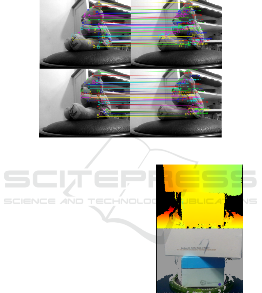
Figure 2: Backtracking.

4 SEGMENTATION

To get a simpliﬁed mesh directly from the scanned

data, we want to ﬁnd the planar area ﬁrst. Taylor and

Cowley (Taylor and Cowley, 2013) use planar area to

identify the wall structure. They use edge detection

and Delaunay triangulation to locate a planar candi-

date. Then, the depth samples associated with each

of the image regions are passed to a RANSAC rou-

tine which is used to recursively divide the point set

into planar regions. Hemmat (Hemmat et al., 2015)

et al. also use edge detection to ﬁnd a region and test

different directions to determine whether their neigh-

borhood is on the same plane or not. Bokaris et al.

(Bokaris et al., 2017) is also similar to Taylor’s ap-

proach, but has better parameters to improve the re-

sult.

An input image may consist of many regions

which are on the same plane. To determine which

pixels belong to the same plane, usually, a RANSAC

algorithm is used. Since a planar area shares the same

normal direction, if we can segment the pixels by

their normal direction, then it will be easier to ﬁnd

the plane. However, this simple idea does not work

correctly. For example, the input image is two planes

as Figure 3 shown. Since the depth value has a quan-

tization error, we have tried different kernel size of

boxes to calculate its mean value to estimate its nor-

mal vector. A larger kernel size can get a smoother

Figure 3: Two planes shown on the input depth and RGB

images.

result. However, the results are still not good as Fig-

ure 4 shown. Because the initial target normal can not

be estimated exactly always, some pixels may belong

to a normal vector and others may belong to another

vector. Thus, the distribution becomes unstable.

To solve the instability problem, a method similar

to the RANSAC algorithm is used. A mask is con-

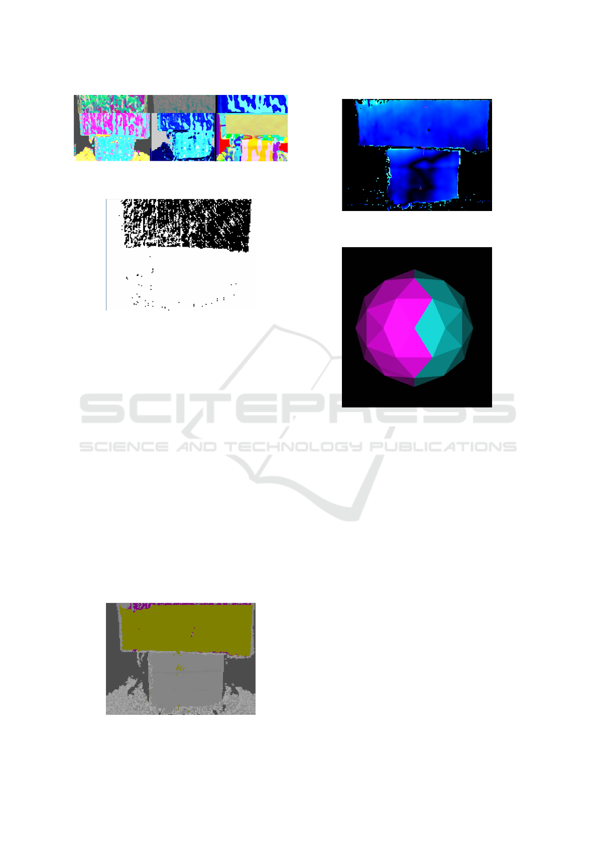
Figure 4: Plane detection is not a stable event with different

sizes of kernel boxes.

Figure 5: A mask represents the pixels that have the com-

mon normal vector.

structed to indicate which pixels that belong to the

same plane can be used to estimate the ﬁtted plane.

The Figure 5 shows the mask. After the parameters

of the plane are estimated, we can check each pixel to

determine whether it belongs to the plane or not. To

label each pixel to a suitable plane, we will calculate

an approximated error by accumulating the distance

from its neighboring pixels to the target plane. If we

only compare the distance, the intersecting area from

another plane also will become a good candidate. To

avoid this situation, we also need to make sure the

variation of the normal vector is similar. The labeling

result is shown on the ﬁgure 6. The error between the

estimated plane and the 3d point from the depth im-

age is shown on the Figure 7. The maximal error is

5mm. The average error is 2 mm.

A curved surface is very different from a planar

surface. The normal vectors of a planar area are the

same or very similar. However, the normal vectors

of a curved area have many differences. Most are

not the same everywhere. Thus, we want to employ

Figure 6: Labeling the pixels belonging to a target plane.

Figure 7: The error between the estimated plane and 3d

points from the depth image.

Figure 8: A subdivision of an Icosahedron is used as an

initial pattern for labeling.

a few planes as ﬁrst patterns to label a depth image

for segmentation. A normal vector from the subdivi-

sion of an Icosahedron is used as the initial pattern as

shown in Figure 8. There are forty triangles for the

half sphere. The angle between the normal vectors of

neighboring triangles is about eighteen degrees.

A mesh structure consists of vertices, edges, and

faces. A vertex determines the geometricsl infor-

mation. An edge is for the topological information.

Mesh simpliﬁcation usually is either by the vertex

decimation method or by the edge collapse approach.

Our approach is trying to minimize the surface num-

ber as much as possible. However, these planes also

are constrained by vertices and edges. Thus, a min-

imal set of vertices are recovered from the domain

graph’s dual graph. To make sure the planar plane

can describe the surface well, tolerance is deﬁned as

follows. Let shape S be described by a mesh M under

a tolerance T . If a point p belongs to a shape S, then

the distance from p to mesh M should be less than T .

To ﬁnd a minimal set of planes to describe a tar-

get surface, a set of primitive planes is deﬁned ﬁrst.

Since all the surfaces face the camera, a half part of a

subdivided icosahedron is suitable as the ﬁrst planes.

For stabilization, each pixel estimates its normal vec-

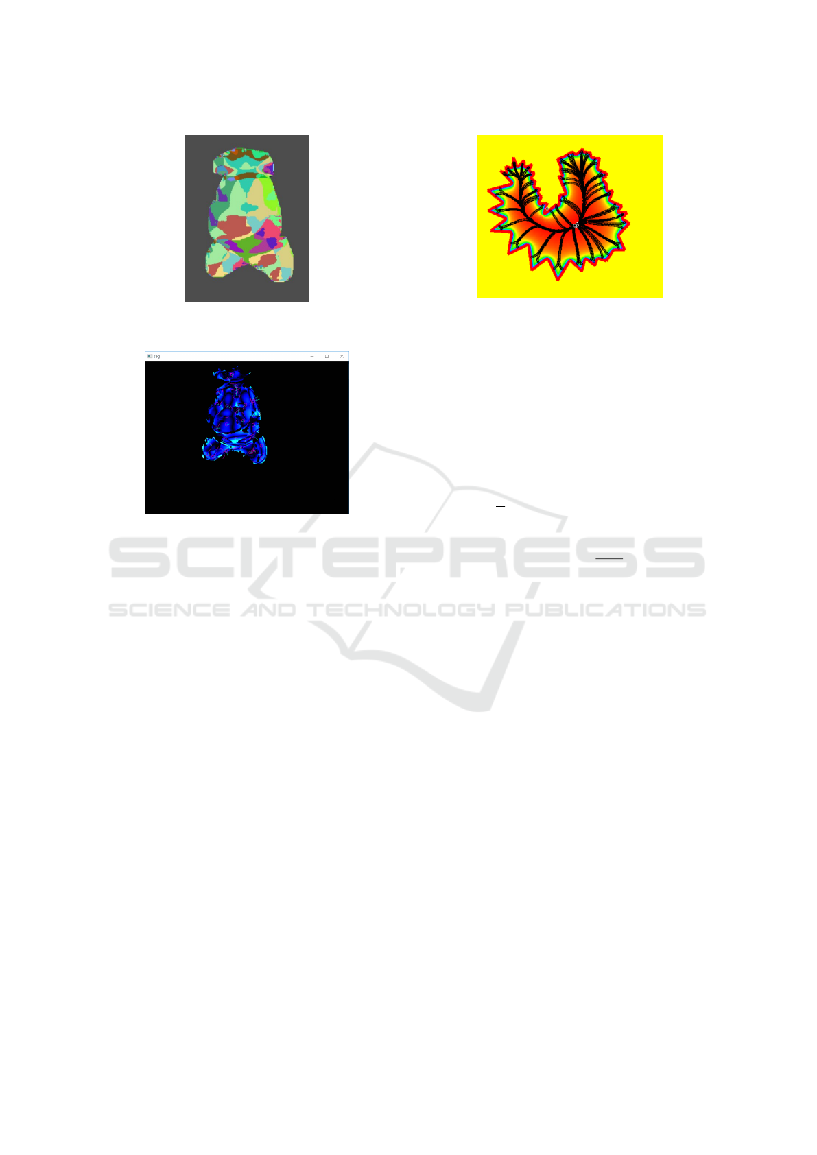
Figure 9: Depth map is segmented by a minimal set of

planes.

Figure 10: The error between an estimated plane and the

depth image for a curved surface.

tor from a seven-by-seven box by comparing the an-

gle between its normal vectors to ﬁnd the best, ﬁttest

primitive plane. Thus, the scanned image can be seg-

mented by labeling with different primitive planes.

For each segmented region, we can ﬁnd its best-ﬁtted

plane. The segmented image is shown in Figure 9.

The error between an estimated plane and the depth

image for a curved surface is shown on Figure 10.

5 DOMAIN SURFACE

To ﬁnd the intersection of two planes, their neighbor-

hood relationship must be deﬁned ﬁrst. For easy iden-

tiﬁcation of the neighborhood relationship, a Dual

graph is constructed from a primitive graph. To con-

struct such a graph, we will ﬁnd some domain nodes

ﬁrst. A domain node represents a critical area in

which every pixel approximates a plane. After an ap-

proximated plane is estimated, each pixel around its

neighbor area will determine whether it belongs to

this plane or not by a predeﬁned threshold. All the

pixels belonging to this plane will form a boundary. A

domain shape is deﬁned, and this shape can determine

some domain nodes. We want to ﬁnd some positions

that are stable and not so sensitive to shape noise. A

domain connected graph seems a good candidate (Wu

Figure 11: The shape shrink into a global optimized posi-

tion even when the shape is very noise.

et al., 2006). It consists of domain nodes. There is

an edge between two domain nodes if there exists a

neighbor relationship.

A domain node is an energy balance position. A

position inside a shape will receive a repulsive force

from its boundary and other domain nodes. A con-

ﬁguration of the boundary will generate a repulsive

force ﬁeld for such a shape. We want to construct a

function that has only one global minimal point in a

convex shape. Thus, a repulsive force ﬁeld is deﬁned

as F(x) =

dθ, where r is the distance from x to

the boundary in the direction~r, and a discrete form is

F(p) =

∑

0≤θ<2π

kpk

, (1)

where ~u

is a unit ray with different angles. When

n → ∞, the repulsive force ﬁeld is dominated by the

shortest distance d(x), and thus f (x) ∝ d(x). In some

sense, n is a term for a smoothing effect. Each po-

sition receives more boundary inﬂuence for a smaller

Let each edge of the shape as an initial position

move to an energy balance position iteratively based

on the repulsive force ﬁeld. Finally, the node will

shrink into a global optimized position that is a do-

main node. Each domain node can generate a max-

imum inscribed circle. This circle will become a

new boundary to reconstruct a repulsive force ﬁeld.

Then, we can ﬁnd all the domain nodes until its ra-

dius smaller than a pre-deﬁned value. The shrinking

process is shown in Figure 11.

Each domain surface maintains a block of the

area. To calculate this area, we will ﬁnd its boundary.

Its boundary is determined by its neighborhood rela-

tionship. Each pixel is labeled with a different code to

represent that it belongs to different domain surface.

Then, we can know to which other surfaces a domain

surface connects. For each pixel on the boundary of

the domain shape, we will check the variation of its

depth or normality among its neighboring pixels to

determine if this point is a continue pixel. If the vari-

ation of depth and normal both are smaller than a pre-

deﬁned constraint, it is a continue pixel. Otherwise,

it is a discrete pixel. Based on the shrinking path on

the domain shape, each boundary segment belongs to

whichever domain node can be determined. Thus, a

continue pixel means that it belongs to two different

domain nodes at its different sides. Also, it means

that the two domain nodes have a neighborhood re-

lationship. A neighborhood edge will be constructed

between the two domain nodes. In other words, for

two neighbor domain surfaces, we can ﬁnd an inter-

section line between these surfaces.

After a domain connected graph is constructed,

each face of the graph helps create vertices. A node

represents a domain face. Thus, a triangle means

that there exists an intersection point of these domain

faces. After traversal of all faces of this graph, we can

construct a list of vertices.

With these vertices, we can reﬁne the boundary

of each domain node. If the boundary is a discrete

edge, then the edge remains unchanged, but if it is a

continuous edge, it will be replaced by a new edge to

connect from the pool of vertices.

If there is a new scan, we should fuse two con-

structed meshes together. Usually, the portion near

the silhouette area is not stable because some of its

neighbors are in the invisible area. For stabilization

reasons, a continuous area should keep its area to at

least a ﬁxed minimum size. A new area will add new

vertices and new edges to the old mesh.

6 REGISTRATION

Pose estimation is an important issue for object scan-

ning or robotic applications. Particularly for object

scanning, the pose is necessary information to fuse

different viewpoints into an integrated model. Mer-

rell et al(Merrell et al., 2007) advocate a two-stage

process in which the ﬁrst stage generates potentially

noisy, overlapping depth maps from a set of calibrated

images and the second stage fuses these depth maps

to obtain an integrated surface with higher accuracy,

suppressed noise, and reduced redundancy.

With a depth camera, the 3d cloud points become

more accessible to capture. Traditionally, there are

two types of approaches. One is based on a set of

known 3d points and their corresponding 2d projec-

tions in the image. It is called the perspective-n-

point (PnP) method. Another type computes the best

matching position by an iterative approach to adjust

to the closest pose. It is called the iterative closest

points(ICP) method.

However, since the estimation of the matching

pairs usually is error-prone, usually massive points

are used to minimize the effect of errors. Some-

times, false matching will produce a huge error. To

remove such outlier effects, the RANSAC (Random

Sample Consensus) Algorithm with an iterative ap-

proach ﬁnds a better ﬁtting. In fact, pose estimation

still does not quickly get a robust result in different

situations. Practically solving this problem, a pre-

calibrated camera array in an environment is more

feasible to recover the pose in different positions. The

other solution may work with the help of an inertial

measurement unit (IMU) to improve the precision.

A speciﬁc area scanned at i-th time forms a do-

main surface f

combined with a region R

and a local

transform M

. The surface ﬁnally will transform into

world coordinates and fuse the global model together.

An array of vertices V

is used to describe a region R

A function f (x)

= n

x + d

where n

is a normal

vector and d

is constant item. A region R

may consist

of domain node c

and f (c

)

= 0.

A global model is

G = ∪M

× R

(2)

We need to ﬁnd at least one motion pair whose

distance is larger than the density check. If a large

transform is found, a pose estimation algorithm will

be used to estimate the object’s pose. To com-

pare different poses, the traditional approach is to

compare shape similarity by calculating the distance

from the depth pixel to the mesh surface, deﬁned as

∑

d(x

,S). Thus, the cost function

E(R,T ) =

∑

d(Rx

+ T, S) (3)

is to be minimized to estimate its transform. How-

ever, in our experiments, the solution is not so robust,

especially in large transform case.

Thus, we will ﬁnd the paired domain surfaces to

estimate the transformation. By the feature tracking

mechanism, a set of paired features can be used to de-

termine the mapping relationship between the domain

surfaces. Assume that surface f

contains feature p

and surface f

contains feature p

. If features p

and

are a mapped pair, then surfaces f

and f

also are a

mapped pair. Then, we can estimate the rotation ma-

trix from the mapped domain surface. Let the normal

vector of the mapped domain surface be n

...n

and n

...n

, respectively. Similar to Sorkine and

Alexa’s research(Sorkine and Alexa, 2007), there ex-

ists a rotation matrix R such that n

= R × n

. To ﬁnd

such a rotation matrix R, we need to minimize

E =

∑

j=1...i

− R × n

(4)

∑

j=1...i

− R × n

)

− R × n

) (5)

∑

j=1...i

)

− 2(n

)

R(n

) + n

(6)

The terms that do not contain R are constant in

the minimization and therefore can be dropped. Thus

remains

argmin

∑

−2(n

)

R(n

) (7)

= argmax

∑

)

R(n

) (8)

= argmax

(R × Tr(

∑

)) (9)

Let S = Tr(

∑

), It is well known that the ro-

tation matrix R maximizing Tr(RS) is obtained when

RS is symmetric positive semi-deﬁnite.

One can derive R from the singular value decom-

position of S = UΣV

R = VU

, (10)

up to changing the sign of the column of U cor-

responding to the smallest singular value, such that

det(R) > 0. After the rotation matrix is determined,

the translation can be obtained by calculating the shift

of feature points.

Here we make a comparison among the PNP, ICP

and domain surface approaches. For different trans-

formations, try to ﬁnd which approach is more robust

and efﬁcient.

7 FUSION

To construct the mesh, a Delaunay triangulation is ap-

plied from the projection plane of the viewpoint, and

the connection of the vertices also can be extended

into three-dimensional space. Each new pose may

create new features that will be added to the exist-

ing mesh. When updating the mesh, each extracted

feature also will compare its distance error to the tol-

erance threshold to determine whether it will be dis-

carded, merged or inserted. When updating the mesh,

each extracted feature also will compare its distance

error to the tolerance threshold. If the distance error

is reasonable and this feature point is far away from

an existing vertex, this feature point will be discarded.

If this feature point is close to an existing vertex, the

vertex position can be updated with a weighted mech-

anism.

P(x) = W ∗ p(X) + w ∗

p(x)

(W +w)

, where p(x) repre-

sents the position of vertex x. Each vertex also main-

tains a weighted value W . Each update also will

change the weight to W = W + w .

If the error is large, that means this feature can

construct a new vertex. If this feature is located out-

side of this mesh, it can be inserted to connect with

the mesh’s boundary vertexes. If this feature is lo-

cated inside the mesh, edges around this new feature

will be checked to delete unsuitable edges. Then, this

vertex can be inserted into the mesh.

Since we focus on object scanning, the texture

map is assumed to be a cubic map. When the ﬁrst

frame creates the mesh, a virtual box around the ob-

ject is also created and the color image will be the

front texture. The u-v relationship also can be found

in accordance with the triangulation result. Each tri-

angle will ﬁnd its best projection plane on the virtual

box. A new update frame also will ﬁnd its best pro-

jection plane to update, and only if the view angle

is closer to the center of the projection plane will its

color image replace the existing frame as the new tex-

ture. All the triangles belonging to that plane need to

update their u-v relationship by projecting their posi-

tion according to that view’s transform.

To fuse two meshes into an integrated mesh, a fu-

sion boundary will be located ﬁrst. Let τ

,τ

be a set

of features that respectively belong to a mesh M

where M

is the integrated mesh and M

is a con-

structed mesh by a new frame. For a particular view,

part of the boundary of M

called B

will divide τ

into two sets τ

,τ

out

. Also, τ

can be divided into two

sets τ

,τ

out

by the mesh M

in the view. B

are the

fusion boundaries on the mesh M

respectively.

In our experience, pose estimation is very impor-

tant. A poor estimation will produce a bad result or

even a mistake. Thus, we need to set a tolerance value

to control the allowable error. The tolerance threshold

cannot be set too low; otherwise, the system will fre-

quently be interrupted because the system cannot get

a good ﬁt to the current model. In general, with our

approach, we can get a textured object model imme-

diately and easily.

8 CONCLUSION

In the beginning, we try to construct the mesh from

features. We want to ﬁnd some invariant features

as candidates and ﬁnd their topological relationship

with Delaunay triangulation. However, silhouette fea-

tures provide an abundance of information, which

also makes it too noisy. Besides, Delaunay triangu-

lation may not ﬁt the variation of depth data. With

the idea of a domain surface, the number of faces be-

comes as few as possible. From the variation of the

mapped area, it is more stable to recover the rotation

transformation. The rigid transformation then can be

divided into the rotation part and the translation part,

and they can be calculated separately. This approach

makes the solution more robust.

ACKNOWLEDGEMENTS

This work was supported in part by the Ministry of

Science and Technology, Taiwan, R.O.C., under grant

no. MOST 106-2221-E-126-011.

REFERENCES

Alexiadis, D. S., Kelly, P., Daras, P., O’Connor, N. E.,

Boubekeur, T., and Moussa, M. B. (2011). Evaluat-

ing a dancer’s performance using kinect-based skele-

ton tracking. In Proceedings of the 19th ACM inter-

national conference on Multimedia, pages 659–662.

ACM.

Bokaris, P.-A., Muselet, D., and Tr

emeau, A. (2017). 3d

reconstruction of indoor scenes using a single rgb-d

image. In 12th International Conference on Computer

Vision Theory and Applications (VISAPP 2017).

Chen, J., Bautembach, D., and Izadi, S. (2013). Scalable

real-time volumetric surface reconstruction. ACM

Transactions on Graphics (TOG), 32(4):113.

Choi, C. and Christensen, H. I. (2016). Rgb-d object pose

estimation in unstructured environments. Robotics

and Autonomous Systems, 75:595–613.

Doulamis, A., Doulamis, N., Ioannidis, C., Chrysouli,

C., Grammalidis, N., Dimitropoulos, K., Potsiou, C.,

Stathopoulou, E. K., and Ioannides, M. (2015). 5d

modelling: an efﬁcient approach for creating spa-

tiotemporal predictive 3d maps of large-scale cul-

tural resources. ISPRS Annals of the Photogramme-

try, Remote Sensing and Spatial Information Sciences,

2(5):61.

Eigen, D. and Fergus, R. (2015). Predicting depth, surface

normals and semantic labels with a common multi-

scale convolutional architecture. In Proceedings of the

IEEE International Conference on Computer Vision,

pages 2650–2658.

Hemmat, H. J., Pourtaherian, A., Bondarev, E., et al. (2015).

Fast planar segmentation of depth images. In Im-

age Processing: Algorithms and Systems XIII, volume

9399, page 93990I. International Society for Optics

and Photonics.

ahler, O., Prisacariu, V. A., Ren, C. Y., Sun, X., Torr, P.,

and Murray, D. (2015). Very high frame rate vol-

umetric integration of depth images on mobile de-

vices. IEEE transactions on visualization and com-

puter graphics, 21(11):1241–1250.

Kainz, B., Hauswiesner, S., Reitmayr, G., Steinberger, M.,

Grasset, R., Gruber, L., Veas, E., Kalkofen, D., Se-

ichter, H., and Schmalstieg, D. (2012). Omnikinect:

real-time dense volumetric data acquisition and appli-

cations. In Proceedings of the 18th ACM symposium

on Virtual reality software and technology, pages 25–

32. ACM.

Keller, M., Leﬂoch, D., Lambers, M., Izadi, S., Weyrich, T.,

and Kolb, A. (2013). Real-time 3d reconstruction in

dynamic scenes using point-based fusion. In 3DTV-

Conference, 2013 International Conference on, pages

1–8. IEEE.

Laggis, A., Doulamis, N., Protopapadakis, E., and Geor-

gopoulos, A. (2017). a low-cost markerless track-

ing system for trajectory interpretation. ISPRS-

International Archives of the Photogrammetry, Re-

mote Sensing and Spatial Information Sciences, pages

413–418.

Leﬂoch, D., Weyrich, T., and Kolb, A. (2015). Anisotropic

point-based fusion. In Information Fusion (Fusion),

2015 18th International Conference on, pages 2121–

2128. IEEE.

Merrell, P., Akbarzadeh, A., Wang, L., Mordohai, P.,

Frahm, J.-M., Yang, R., Nist

er, D., and Pollefeys,

M. (2007). Real-time visibility-based fusion of depth

maps. In Computer Vision, 2007. ICCV 2007. IEEE

11th International Conference on, pages 1–8. IEEE.

Newcombe, R. A., Izadi, S., Hilliges, O., Molyneaux, D.,

Kim, D., Davison, A. J., Kohi, P., Shotton, J., Hodges,

S., and Fitzgibbon, A. (2011). Kinectfusion: Real-

time dense surface mapping and tracking. In 2011

10th IEEE International Symposium on Mixed and

Augmented Reality, pages 127–136.

Nießner, M., Zollh

ofer, M., Izadi, S., and Stamminger,

M. (2013). Real-time 3d reconstruction at scale us-

ing voxel hashing. ACM Transactions on Graphics

(TOG), 32(6):169.

Ondr

ska, P., Kohli, P., and Izadi, S. (2015). Mo-

bilefusion: Real-time volumetric surface reconstruc-

tion and dense tracking on mobile phones. IEEE

transactions on visualization and computer graphics,

21(11):1251–1258.

Papadopoulos, G. T., Axenopoulos, A., and Daras, P.

(2014). Real-time skeleton-tracking-based human ac-

tion recognition using kinect data. In MMM (1), pages

473–483.

Papazov, C., Marks, T. K., and Jones, M. (2015). Real-time

3d head pose and facial landmark estimation from

depth images using triangular surface patch features.

In Proceedings of the IEEE conference on computer

vision and pattern recognition, pages 4722–4730.

Pradeep, V., Rhemann, C., Izadi, S., Zach, C., Bleyer,

M., and Bathiche, S. (2013). Monofusion: Real-time

3d reconstruction of small scenes with a single web

camera. In Mixed and Augmented Reality (ISMAR),

2013 IEEE International Symposium on, pages 83–88.

IEEE.

Salas-Moreno, R. F., Newcombe, R. A., Strasdat, H., Kelly,

P. H., and Davison, A. J. (2013). Slam++: Simulta-

neous localisation and mapping at the level of objects.

In Proceedings of the IEEE conference on computer

vision and pattern recognition, pages 1352–1359.

Sorkine, O. and Alexa, M. (2007). As-rigid-as-possible sur-

face modeling. In Symposium on Geometry process-

ing, volume 4.

Taylor, C. J. and Cowley, A. (2013). Parsing indoor scenes

using rgb-d imagery. In Robotics: Science and Sys-

tems, volume 8, pages 401–408.

Whelan, T., Johannsson, H., Kaess, M., Leonard, J. J., and

McDonald, J. (2013). Robust real-time visual odome-

try for dense rgb-d mapping. In Robotics and Automa-

tion (ICRA), 2013 IEEE International Conference on,

pages 5724–5731. IEEE.

Whelan, T., Kaess, M., Fallon, M., Johannsson, H.,

Leonard, J., and McDonald, J. (2012). Kintinuous:

Spatially extended kinectfusion.

Wu, F.-C., Ma, W.-C., Liang, R.-H., Chen, B.-Y., and Ouhy-

oung, M. (2006). Domain connected graph: the skele-

ton of a closed 3d shape for animation. The Visual

Computer, 22(2):117–135.

Zeng, M., Zhao, F., Zheng, J., and Liu, X. (2013). Octree-

based fusion for realtime 3d reconstruction. Graphical

Models, 75(3):126–136.

Zollh

ofer, M., Nießner, M., Izadi, S., Rehmann, C., Zach,

C., Fisher, M., Wu, C., Fitzgibbon, A., Loop, C.,

Theobalt, C., et al. (2014). Real-time non-rigid recon-

struction using an rgb-d camera. ACM Transactions

on Graphics (TOG), 33(4):156.