Towards Combining Reactive and Proactive Cloud Elasticity on Running
HPC Applications
Vinicius Facco Rodrigues
1
, Rodrigo da Rosa Righi
1
, Cristiano Andr
´
e da Costa
1
, Dhananjay Singh
2
,
Victor Mendez Munoz
3
and Victor Chang
4
1
Applied Computing Graduate Program, Universidade do Vale do Rio dos Sinos (UNISINOS), Brazil
2
Hankuk Univeristy of Foreign Studies (HUFS), Republic of Korea
3
Autonomous University of Barcelona, Barcelona, Spain
4
Xi’an Jiaotong Liverpool University, Suzhou, China
Keywords:
Cloud Utility, High-performance Computing, Live Thresholding, Resource Management, Self-organizing.
Abstract:
The elasticity feature of cloud computing has been proved as pertinent for parallel applications, since users do
not need to take care about the best choice for the number of processes/resources beforehand. To accomplish
this, the most common approaches use threshold-based reactive elasticity or time-consuming proactive elas-
ticity. However, both present at least one problem related to: the need of a previous user experience, lack on
handling load peaks, completion of parameters or design for a specific infrastructure and workload setting. In
this regard, we developed a hybrid elasticity service for parallel applications named SelfElastic. As parameter-
less model, SelfElastic presents a closed control loop elasticity architecture that adapts at runtime the values
of lower and upper thresholds. Besides presenting SelfElastic, our purpose is to provide a comparison with
our previous work on reactive elasticity called AutoElastic. The results present the SelfElastic’s lightweight
feature, besides highlighting its performance competitiveness in terms of application time and cost metrics.
1 INTRODUCTION
Commonly, HPC applications are executed either on
clusters or grid architectures. Maintaining these en-
vironments in terms of infrastructure, scheduling, and
energy consumption may turn it an expensive solu-
tion (Niu et al., 2013). In the HPC view point, a
shared characteristic of such environments regards the
fixed number of resources to run an application. Due
this limitation, deciding the right amount of processes
to execute an HPC application can be a difficult pro-
cedure. Conversely, cloud computing has been gai-
ning attention in this context thanks to its resource
reorganization facility named elasticity (Herbst et al.,
2015), which The act of deciding the right amount
of cloud computing resources for a parallel applica-
tion is a nontrivial task and may lead to either under-
provisioning or over-provisioning (Nikravesh et al.,
2015; Dustdar et al., 2015). Today, most of the elasti-
city control strategies can be classified as either being
reactive or proactive (Farokhi et al., 2015; Nikravesh
et al., 2015; Moore et al., 2013). For the first case,
typically users define an upper bound t
u
and a lo-
wer bound t
l
in an ad-hoc manner on a target per-
formance metric to trigger, respectively, the activa-
tion and deactivation of a certain number of resour-
ces (Netto et al., 2014). On the other hand, a pro-
active approach employs prediction techniques to an-
ticipate the behavior of the system (its load) and the-
reby decide the reconfiguration actions. The afore-
mentioned requirements are not trivial and someti-
mes is needed a deep knowledge about the behavior
of the system over time (Dustdar et al., 2015; Jams-
hidi et al., 2014). In this context, we have proposed
in previous work a model named AutoElastic (Righi
et al., 2015a; Righi et al., 2015b; Righi et al., 2016)
which addresses reactive elasticity to reorganize re-
sources for loop-based synchronous parallel applica-
tions. Although achieving remarkable performance
gains, AutoElastic remains suffering the main pro-
blems of reactive elasticity approaches: definition of
thresholds and reactivity. In this context, this arti-
cle presents a new elasticity model called SefElas-
tic, which offers automatic threshold configuration.
SelfElastic presents the following contributions to the
state-of-the-art when considering the HPC applicati-
ons and cloud elasticity duet: (i) a modeling of clo-
Facco Rodrigues, V., Righi, R., André da Costa, C., Singh, D., Munoz, V. and Chang, V.
Towards Combining Reactive and Proactive Cloud Elasticity on Running HPC Applications.
DOI: 10.5220/0006761302610268
In Proceedings of the 3rd International Conference on Internet of Things, Big Data and Security (IoTBDS 2018), pages 261-268
ISBN: 978-989-758-296-7
Copyright
c
 2019 by SCITEPRESS – Science and Technology Publications, Lda. All rights reserved
261

sed control-theoretic (Ghanbari et al., 2011) infra-
structure to support the hybrid elasticity behavior on
parallel cloud-based applications; and (ii) based on
the TCP (Transmission Control Protocol) congestion
control, we propose an algorithm named Live Thres-
holding (LT) to handle application load projection and
lower and upper thresholds adaptivity.
2 RELATED WORK
Today, we can cite basically two main types of appli-
cation workloads that could take profit from elasticity
in the cloud (Ghanbari et al., 2011): (i) transactio-
nal (Moore et al., 2013; Nikolov et al., 2014); and (ii)
batch (e.g., text mining, video transcoding, graphical
rendering and parallel applications) (Niu et al., 2013;
Righi et al., 2015a). The applications in the first case
are built to serve online HTTP clients, being com-
monly deployed on commercial systems like Amazon
AWS, RightScale and Microsoft Azure using reactive
elasticity (Nikravesh et al., 2015). Users must com-
plete the rules and the limits of a metric to be mo-
nitored as well as the conditions and actions for re-
configuration. Besides graphical and command-line
tools, these commercial systems also provide a parti-
cular API for resource provisioning and monitoring.
Reactive elasticity is explored in two scenarios: (i)
when using the standard technique with static thres-
holds (Dustdar et al., 2015; Righi et al., 2015a; Righi
et al., 2015b; Righi et al., 2016; Galante and Bona,
2015); (ii) when using other techniques to runtime
adapt the threshold values (Netto et al., 2014). In
both scenarios, there are at least a lower (t
l
) and an
upper (t
u
) threshold that guide horizontal or vertical
elasticity. It is unison among the authors that the per-
formance of the threshold-based technique is highly
dependent on the selected parameters, even in the se-
cond scenario (Farokhi et al., 2015). In addition to
performance, energy consumption and cost metrics
are also important both at user and cloud administra-
tor perspectives (Righi et al., 2016). Other problems
are related to reactiveness to trigger elasticity actions
and oscillations on VM allocations.
3 SelfElastic MODEL
We developed SelfElastic with the following design
decisions in mind: (i) parameterless, not needing
to write elasticity rules, conditions or thresholds at
user/programmer perspective; (ii) easy-to-use elas-
ticity service, being provided in a plug-and-play
fashion; (iii) without needing any prior information
about the application components/phases and without
needing previous executions to generate metadata;
(iv) lightweight, so not being prohibitive for time-
sensitive HPC applications; (v) easy integration with
the parallel application, so the processes can be reor-
ganized easily and quickly in the presence of a drop
or addition of resources.
3.1 Closed Feedback-Loop Architecture
Aiming at providing a proactive feature, we desig-
ned SelfElastic as a closed feedback-loop architec-
ture (Ghanbari et al., 2011), involving two main
components: the SelfElastic Manager and the cloud,
which is our target system. As illustrated in Figure 1,
we have a loop in which the monitoring metrics serve
to optimize and predict internal parameters, so trigge-
ring or not elasticity actions to support the application
historical behavior.
P P
Node 0
Node m-1
Cloud
front-end
Data
Shared
Area
Physical Layer
Virtual Layer
VM
0
VM
c-1
VM
n-1
VM
(m-1) x c
...
...
P P
Application Layer
Cloud
Legend
SelfElastic Manager
Actuator: Elasticity
Actions
Controller: Live
Thresholding and
System Load
Sensor:
Monitoring
Switch
P
Application Process
VM
Virtual Machine
...
Figure 1: SelfElastic architecture, with two main compo-
nents: SelfElastic Manager and a cloud-based parallel ap-
plication (our target system). At the cloud perspective, c
denotes the number of cores inside a node, m is the num-
ber of nodes and n refers to the number of VMs running
application processes, being obtained by c × m.
Our cloud model considers a front-end that acts as
a cloud manager to instantiate, deallocate and monitor
VMs in the Virtual Layer and a set of homogeneous
nodes in the Physical Layer. In addition, the front-end
also accounts for answering requests (including the
three previous procedures) done with the cloud API
by the SelfElastic Manager. Regarding the Applica-
tion Layer, there is a collection of processes which
are instantiated through application-specific VM tem-
plates. Each VM is assigned with an template and au-
tomatically starts an application process. Depending
on the application, different VM templates could start
processes with distinct functions.
3.2 Defining the Notion of System Load
The sensor module of SelfElastic Manager monitors
CPU load of each VM periodically, passing data to
the controller afterward. In turn, the controller apply
IoTBDS 2018 - 3rd International Conference on Internet of Things, Big Data and Security
262

algorithms to define load and threshold values. If re-
source reorganization is necessary, the actuator pro-
ceeds elasticity actions using the cloud API. When
completing tasks of all modules, the SelfElastic Ma-
nager ends a monitoring observation and waits for
the next monitoring cycle. One role of the control-
ler is to generate the system load (l) in order to mi-
nimize the effect of disturbances or noises on the be-
havior of the target system. Thus, we are working
with time-series and SES (Simple Exponential Smoo-
thing (Herbst et al., 2013)) technique over the CPU
load metric of each VM. Equation 1 presents l(o) as
the system load at the o
th
monitoring observation con-
sidering n active VMs. This equation is an arithme-
tic average of the load on each VM, which is com-
puted through l
0
(v, o). Here, v is a VM index, o is
the current monitoring observation and n the number
of VMs running application processes (see Equation
2). l
0
consists in a SES average, where the weight
of the current observation o has a stronger influence
than o−1 in the final calculus (starting from
1
2
, we are
using
1
4
,
1
8
an so on for the weights). The recurrence
ends in the cpu(v, o) computation, which returns the
CPU load of VM v at observation o.
l(o) =
∑
n−1
v=0
l
0
(v, o)
n
(1)
l
0
(v, o) =



cpu(v,o)
2
i f o = 0
l
0
(v,o−1)
2
+
cpu(v,o)
2
i f o 6= 0
(2)
3.3 Live Thresholding Technique
The Manager is responsible for retrieving a vector
of CPU load from all VMs running slave proces-
ses. More precisely, the sensor module of the Ma-
nager periodically queries the cloud front-end to cap-
ture such data. The mentioned vector is used to
compute the system load detailed in Subsection 3.2.
Instead of using static thresholds, SelfElastic propo-
ses the dynamic adaption of the lower (t
l
) and upper
(t
u
) thresholds, which are initiated with the values 0
and 100, respectively. We named this novel techni-
que as Live Thresholding (LT), which considers the
definition of two procedures: adapt thresholds() and
reset thresholds(). The former is computed at each
monitoring observation, while the second is called
only when an elasticity action takes place.
adaptT hresholds() has three parameters: t
l
, t
u
(both input/output) and load (only input). Firstly, we
compute the system load variation considering both
current and previous monitoring observations (refer-
red by the indexes o and o − 1, respectively). This
value is assigned to ∆l (Equation 3), where function
l() was defined earlier in Subsection 3.2. ∆l decides
which threshold will be updated: (i) if ∆l is negative,
we are experiencing a decreasing load behavior so t
l
is recalculated to handle this situation quickly; (ii) if
∆l is positive, the application workload is growing up
so t
u
is updated to address this situation; (iii) if ∆l is
equal to 0, threshold adaptations do not occur. Equa-
tions 4 and 5 present how new values of thresholds
are computed. Contemplating that t
u
decreases when
updated, it has a lower bound equal to 0. On the other
side, an upper bound of 100 is used when computing
the new value of t
l
.
∆l = l(o)− l(o − 1) (3)
t
l
= Min(t
l
+ |∆l|, 100) (4)
t
u
= Max(t
u
− ∆l, 0) (5)
An initial thought to design the resetT hresholds()
procedure, which has the same set of parameters pre-
sented in adaptT hresholds(), is to reassign these de-
fault values at each elasticity action. In our understan-
ding, this threshold resetting strategy may not be the
best for elasticity reactivity, since we are putting away
all historical data stored in the SelfElastic Manager.
Aiming at proposing new forms to reset thresholds,
we analyzed the TCP congestion algorithm (Bing
et al., 2009). In the TCP protocol, after exceeding
a threshold, the window value is incremented linearly
by the maximum segment at each burst. So, at each
timeout, this threshold is set to half of the current con-
gestion window, and the congestion window is reset
to one maximum segment. Thus, we have investiga-
ted 6 approaches A
z
(A
z
|z ∈ {a, b, c, d, e, f }) to address
threshold adaptivity after an elasticity action:
• When violating t
l
we can apply A
a
, A
b
or A
c
in
accordance with Equation 6 to compute the new
value for t
l
, while t
u
is redefined to 100;
• When violating t
u
we can apply A
d
, A
e
or A
f
in
accordance with Equation 7 to compute the new
value of t
u
, while t
l
is restarted as 0.
t
l
=













0 f or A
a
l (o)
2
f or A
b
l(o − 1) −



l (o−1)−l(o)
2



f or A
c
(6)
t
u
=













100 f or A
d
l(o) +
100−l(o)
2
f or A
e
l(o − 1) +



l (o−1)−l(o)
2



f or A
f
(7)
SelfElastic always uses a fixed combination of one
approach when violating t
l
and another for t
u
. This re-
sults in a notation named LT
xy
, where x (x is A
a
, A
b
or
Towards Combining Reactive and Proactive Cloud Elasticity on Running HPC Applications
263

A
c
) and y (y is A
d
, A
e
or A
f
) refer to a particular possi-
bility for the lower and upper thresholds, respectively.
A
a
and A
d
simply reset the thresholds to the same va-
lues that they were initialized when starting the moni-
toring. A
b
and A
e
use the system load after an elasti-
city action to redesign the thresholds, while A
c
and A
f
achieve them considering the system load before and
after delivering/consolidating resources. SelfElastic
is a parameterless model, so the possibility to choose
elasticity approaches does not fit our previous design
decision. In this way, we conducted experiments with
all possibilities of LT
xy
over eight load patterns consi-
dered in the evaluation methodology.
4 EVALUATION
METHODOLOGY
We developed a master-slave HPC iterative appli-
cation that computes the numerical integration of a
function f (x) in a closed interval [a, b]. The appli-
cation presents a master process that works in an ex-
ternal loop, where it reads a line from a file that de-
fines the current workload for such an iteration and
the number of them. Figure 2 presents the eight lo-
ads patterns. To evaluate all LT strategies we fir-
stly executed all combinations of LT
xy
with the ap-
plication running the load patterns Constant, Ascen-
ding, Descending and Wave. From this evaluation we
analyzed the best choice for LT to be considered in
the next experiments. All eight loads were executed
in three different scenarios: (s1) without cloud elas-
ticity; (s2) enabling self-organizing elasticity mana-
gement through the functioning of the LT technique;
(s3) traditional elasticity approach using static thres-
holds. While SelfElastic is employed to accomplish
the second scenario, our previous work named Au-
toElastic (Righi et al., 2015a) is adopted to address
the third one. Contrary to AutoElastic, here we are
using 4 combinations of thresholds: t
l
30% and 50%;
and t
u
70% and 90%. Additionaly, our evaluation ana-
lyzes the load patterns and the scenarios against three
metrics: time, resource and cost.
5 EVALUATION
In this section, we firstly present in Subsection 5.1
an analysis of the cloud and behavior with elasticity
guided by all LT ideas. Then, in Subsection 5.2 we
focus on evaluating the best strategy for LT . In Sub-
section 5.3 we analyze the application performance.
0 500
10000
0
1000000
equation
subintervals
(s)
(a)
0 500
10000
0
1000000
equation
subintervals
(s)
(b)
0 500
10000
0
1000000
equation
subintervals
(s)
(c)
0 500
10000
0
1000000
equation
subintervals
(s)
(d)
0 500
10000
0
8000000
equation
subintervals
(s)
(e)
0 500
10000
0
8000000
equation
subintervals
(s)
(f)
0 500
10000
0
1000000
equation
subintervals
(s)
(g)
0 500
10000
0
1000000
equation
subintervals
(s)
(h)
Figure 2: Eight workload patterns considered in the tests:
(a) Constant; (b) Ascending; (c) Descending; (d) Wave; (e)
Positive Exponential; (f) Negative Exponential; (g) Partial
Random; (h)Total Random.
5.1 Analyzing Behavior of the LT
Technique
Figure 3 shows all application executions with the
Constant load. In this load, violations in the lower
threshold (t
l
) did not occur. The tiny variations in the
load bring similar adaptions in both thresholds. Ho-
wever, t
u
is always violated resulting in addition of
resources since the load always range the same va-
lues and it is nearer the upper threshold (t
u
). The fi-
gures (b), (e) and (h) present the common use of the
A
e
approach. In these executions, when an elasticity
action was performed, t
u
was recalculated to a new
value close to the load. It resulted in new violations
faster than the other strategies.
The Figure 4 presents LT when executing the As-
cending load pattern. As occurred in the Constant
load, here the t
l
was not violated since the load has a
growing trend. In this way, figures (b), (c), (e), (f), (h)
and (i) where strategies recalculated the t
u
to values
near the load, resulted in higher resource consumption
and lower execution times. Particularly, executions
with the A
f
approach achieved up to 12 VMs resulting
in faster executions. However, even though in figure
(h) the maximum of resources was 10 VMs, this exe-
cution achieved the best result considering time. It
happened because resources were added faster in the
beginning of the execution when comparing with the
other approaches. So, with more resources availa-
ble earlier, the application ended without needing two
more extra resources.
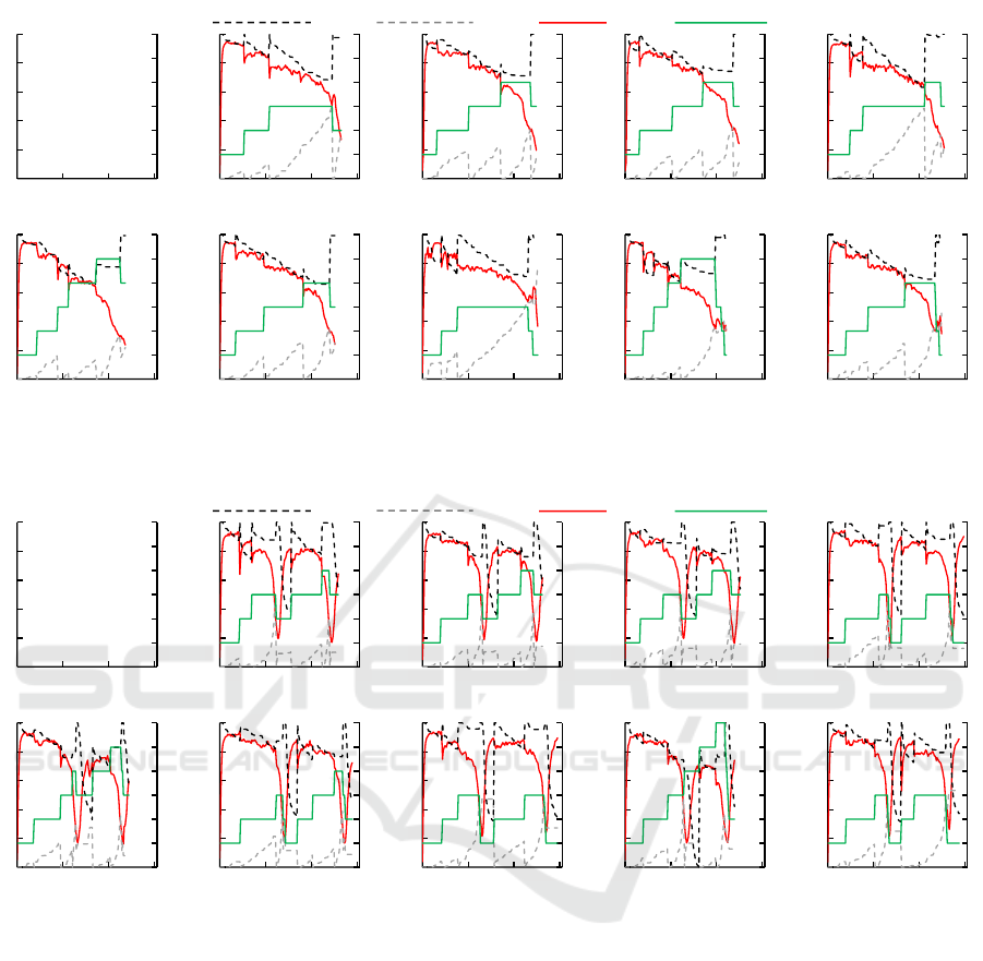
Figure 5 present the behavior of the cloud with the
application running with the Descending load pattern.
This load has an opposite trend when comparing with
the Ascending load. In this way, differently from the
loads Constant and Ascending, here t
l
has impact in
elasticity actions. In addition, as the load started in a
high level and decreased slowly, it violated the t
u
in all
IoTBDS 2018 - 3rd International Conference on Internet of Things, Big Data and Security
264

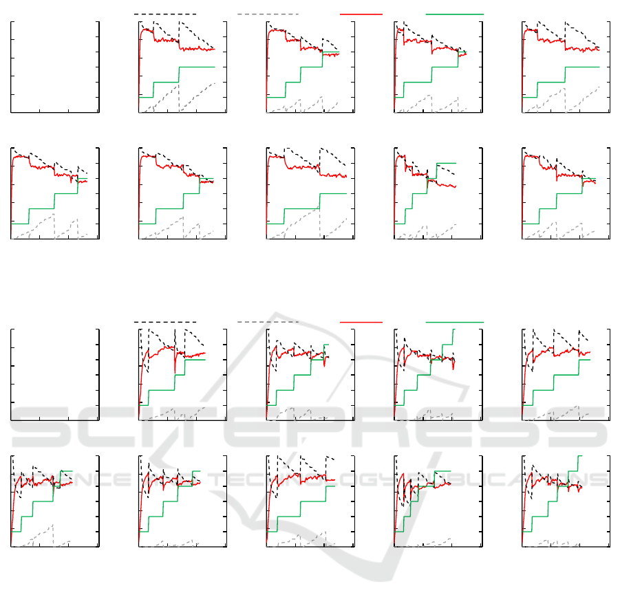
Upper Threshold
Lower Threshold
Cloud Load Virtual Machines
load
virtual machines
time (seconds)
Axis legends
0 0.2 0.4 0.6 0.8 1
0 900 1800 2700
12 10 8 6 4
2
0
(a) LT
ad
0 0.2 0.4 0.6 0.8 1
0 900 1800 2700
12 10 8 6 4
2
0
(b) LT
ae
0 0.2 0.4 0.6 0.8 1
0 900 1800 2700
12 10 8 6 4
2
0
(c) LT
a f
0 0.2 0.4 0.6 0.8 1
0 900 1800 2700
12 10 8 6 4
2
0
(d) LT
bd
0 0.2 0.4 0.6 0.8 1
0 900 1800 2700
12 10 8 6 4
2
0
(e) LT
be
0 0.2 0.4 0.6 0.8 1
0 900 1800 2700
12 10 8 6 4
2
0
(f) LT
b f
0 0.2 0.4 0.6 0.8 1
0 900 1800 2700
12 10 8 6 4
2
0
(g) LT
cd
0 0.2 0.4 0.6 0.8 1
0 900 1800 2700
12 10 8 6 4
2
0
(h) LT
ce
0 0.2 0.4 0.6 0.8 1
0 900 1800 2700
12 10 8 6 4
2
0
(i) LT
c f
Figure 3: Historical behavior of cloud parameters and resources when running the application with the Constant load.
Upper Threshold
Lower Threshold
Cloud Load Virtual Machines
load
virtual machines
time (seconds)
Axis legends
0 0.2 0.4 0.6 0.8 1
0 900 1800 2700
12 10 8 6 4
2
0
(a) LT
ad
0 0.2 0.4 0.6 0.8 1
0 900 1800 2700
12 10 8 6 4
2
0
(b) LT
ae
0 0.2 0.4 0.6 0.8 1
0 900 1800 2700
12 10 8 6 4
2
0
(c) LT
a f
0 0.2 0.4 0.6 0.8 1
0 900 1800 2700
12 10 8 6 4
2
0
(d) LT
bd
0 0.2 0.4 0.6 0.8 1
0 900 1800 2700
12 10 8 6 4
2
0
(e) LT
be
0 0.2 0.4 0.6 0.8 1
0 900 1800 2700
12 10 8 6 4
2
0
(f) LT
b f
0 0.2 0.4 0.6 0.8 1
0 900 1800 2700
12 10 8 6 4
2
0
(g) LT
cd
0 0.2 0.4 0.6 0.8 1
0 900 1800 2700
12 10 8 6 4
2
0
(h) LT
ce
0 0.2 0.4 0.6 0.8 1
0 900 1800 2700
12 10 8 6 4
2
0
(i) LT
c f
Figure 4: Historical behavior of cloud parameters and resources when running the application with the Ascending load.
executions. The LT technique is sensible to small va-
riations in the load, thus t
u
decreased hitting the load
and it resulted in addition of resources. The first half
of execution impacted in performance more than the
final part. Resources were added to the cloud in this
phase where the load were in high levels. When it
started do decrease, in all executions the t
l
were vio-
lated when the application was near the end. This do
not had great impact in performance because the time
the application executed with a set new with less re-
sources were to small.
Finally, Figure 6 presents the executions with all
LT combinations running the Wave load pattern. In
this scenario, both t
l
and t
u
were violated resulting in
elasticity actions. Figures (a), (b) and (c) present si-
milar behaviors and the common use of the strategy
A
a
. The variation of the strategy to recalculate t
u
cau-
sed variations only in the time when new resources
were added. In scenarios presented by figures (d), (e)
and (f) the amount of resources available was diffe-
rent in each one. The main difference occurred in (e)
since extra resources were added when the load were
decreasing near 1000 seconds. It happened because
a new elasticity action was already started before and
resources were available only at this point. With this
extra resources the application execute faster in the
last portion of time, resulting in a better performance.
Likewise, figures (g), (h) and (i) present LT applying
A
c
and differing the strategy to recalculate t
u
. Fi-
gure (h) presents a behavior quite different than the
Towards Combining Reactive and Proactive Cloud Elasticity on Running HPC Applications
265

Upper Threshold
Lower Threshold
Cloud Load Virtual Machines
load
virtual machines
time (seconds)
Axis legends
0 0.2 0.4 0.6 0.8 1
0 900 1800 2700
12 10 8 6 4
2
0
(a) LT
ad
0 0.2 0.4 0.6 0.8 1
0 900 1800 2700
12 10 8 6 4
2
0
(b) LT
ae
0 0.2 0.4 0.6 0.8 1
0 900 1800 2700
12 10 8 6 4
2
0
(c) LT
a f
0 0.2 0.4 0.6 0.8 1
0 900 1800 2700
12 10 8 6 4
2
0
(d) LT
bd
0 0.2 0.4 0.6 0.8 1
0 900 1800 2700
12 10 8 6 4
2
0
(e) LT
be
0 0.2 0.4 0.6 0.8 1
0 900 1800 2700
12 10 8 6 4
2
0
(f) LT
b f
0 0.2 0.4 0.6 0.8 1
0 900 1800 2700
12 10 8 6 4
2
0
(g) LT
cd
0 0.2 0.4 0.6 0.8 1
0 900 1800 2700
12 10 8 6 4
2
0
(h) LT
ce
0 0.2 0.4 0.6 0.8 1
0 900 1800 2700
12 10 8 6 4
2
0
(i) LT
c f
Figure 5: Historical behavior of cloud parameters and resources when running the application with the Descending load.
Upper Threshold
Lower Threshold
Cloud Load Virtual Machines
load
virtual machines
time (seconds)
Axis legends
0 0.2 0.4 0.6 0.8 1
0 900 1800 2700
12 10 8 6 4
2
0
(a) LT
ad
0 0.2 0.4 0.6 0.8 1
0 900 1800 2700
12 10 8 6 4
2
0
(b) LT
ae
0 0.2 0.4 0.6 0.8 1
0 900 1800 2700
12 10 8 6 4
2
0
(c) LT
a f
0 0.2 0.4 0.6 0.8 1
0 900 1800 2700
12 10 8 6 4
2
0
(d) LT
bd
0 0.2 0.4 0.6 0.8 1
0 900 1800 2700
12 10 8 6 4
2
0
(e) LT
be
0 0.2 0.4 0.6 0.8 1
0 900 1800 2700
12 10 8 6 4
2
0
(f) LT
b f
0 0.2 0.4 0.6 0.8 1
0 900 1800 2700
12 10 8 6 4
2
0
(g) LT
cd
0 0.2 0.4 0.6 0.8 1
0 900 1800 2700
12 10 8 6 4
2
0
(h) LT
ce
0 0.2 0.4 0.6 0.8 1
0 900 1800 2700
12 10 8 6 4
2
0
(i) LT
c f
Figure 6: Historical behavior of cloud parameters and resources when running the application with the Wave load.
others two. While in (g) and (i) two elasticity acti-
ons were performed to remove resources in the first
load drop, in (h) it did no occur. It happened because
when the load started to drop by the time 1000 se-
conds an elasticity action to increase resources was
already running. As SelfElastic does not trigger si-
multaneously elasticity actions, new actions were al-
lowed only when this new resources were available.
However, it happened after the load drop and when
the application load was already increasing again. As
the application keep resources from former actions,
the second half of execution was faster in this scena-
rio than all other scenarios.
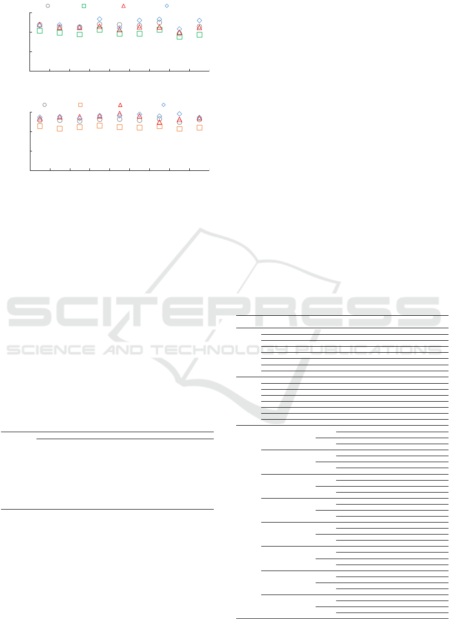
5.2 Defining Final Approach for LT
Figure 7 presents results of the metrics time (a) and
cost (b) when executing the load patterns Constant,
Ascending, Descending and Wave with all possibili-
ties for LT . In the time perspective, Figure 7 (a) shows
that LT
ce
achieved better results than the other approa-
ches. This strategy obtained the best mean time (1967
seconds) between all four loads. Although pertinent
for performance purposes, we cannot negligence re-
source consumption and consequently the cost me-
tric. When analyzing cost, the gains of LT
ce
are not
so evident in Figure 7 (b). However, this strategy also
obtained the best mean of all loads costs.
Aiming at generating a single approach to guide
IoTBDS 2018 - 3rd International Conference on Internet of Things, Big Data and Security
266

0
1000
2000
3000
LTad LTae LTaf LTbd LTbe LTbf LTcd LTce LTcf
Time (
seconds
)
Constant Ascending Descending Wave
(a) Execution Time
0 10000
20000
30000
LTad LTae LTaf LTbd LTbe LTbf LTcd LTce LTcf
Cost [x1000]
Constant Ascending Descending Wave
(b) Cost
Figure 7: Results of metrics (a) time and (b) cost when run-
ning the load patterns.
the functioning of the Live Thresholding technique,
we used the cost within the Weighted Sum Mo-
del (Triantaphyllou, 2000) techique. Therefore, for
each load pattern we classified the cost results of the
nine combinations of LT
xy
in an ascending fashion.
For each one we attributed a weight starting from 1.0
for the first place, 0.9 for the second, 0.8 for the third
and so on. Thus, considering we have executed all
nine LT combinations with four load patterns, each
LT
xy
received four weights. So then, the sum of them
represents the final result where the highest value de-
fines the final approach for LT . Table 1 shows this
evaluation revealing LT
ce
as the better strategy for LT .
Table 1: Using the cost metric to define the final solution
for the Live Thresholding: LT
ce
was selected as the best
approach when combining different types of work loads.
LT
xy
Weight
Ascending Constant Descending Wave Total
LT
ad
0.3 0.7 0.8 0.8 2.6
LT
ae
0.9 0.8 0.6 0.7 3.0
LT
a f
0.5 0.9 0.5 1.0 2.9
LT
bd
0.2 0.4 0.3 0.4 1.3
LT
be
0.6 0.3 0.2 0.5 1.6
LT
b f
0.7 0.6 0.4 0.3 2.0
LT
cd
0.4 0.2 1.0 0.6 2.2
LT
ce
1.0 1.0 0.9 0.2 3.1
LT
c f
0.8 0.5 0.7 0.9 2.9
5.3 Performance Analysis
Table 2 shows results we obtained running the appli-
cation with all load patterns and parameters. For the
scenario s2, the results regards to the strategy LT
ce
which is the one we adopted as final in Subsection 5.2.
For simplicity, here we will call LT
ce
just LT . One of
the differences between LT and approaches with sta-
tic thresholds regards to how each strategy behaviors
at the exact moment after a resource reorganization.
In the best case for static thresholds, lower values for
t
u
and higher values for t
l
increases reactivity. In these
cases, when the load drops or increases after an ope-
ration it can stay over or under the same threshold
that has triggered the last operation. For this reason,
a new operation can occur sooner and it can antici-
pate actions. Conversely, in the worst case, higher va-
lues for t
u
and lower values for t
l
decreases reactivity
since the load could stagnate between the thresholds
not allowing more operations. In addition, with lo-
ads trending up or down, in these situations after an
operation it could take more time to the load reach
a threshold again. Differently from static thresholds,
LT proposes an algorithm to recalculate both t
u
and t
l
after an elasticity operation to close the load after the
operation. Thus, elasticity actions do not occur in the
observation that the thresholds are recalculated. It ta-
kes some more observations do continue adapting the
thresholds and then violate it again. In most results,
this distinct behavior made LT achieve time and cost
values slightly higher then the ones the better set of
static thresholds achieved. On the other hand, it also
made LT achieve results much better than the ones
obtained by the worst set of thresholds.
Table 2: Results of all scenarios and metrics.
Scenario Application Pattern
Thresholds
Time Resource Cost
t
u
t
l
s1 Without Elasticity
Ascending - - 4319 8618 37221142
Descending - - 4410 8798 38799180
Constant - - 4283 8542 36585386
Wave - - 4363 8700 37958100
Pos. Exponential - - 4601 9180 42237180
Neg. Exponential - - 4528 9042 40942176
All Random - - 4018 8040 32304720
Partial Random - - 3994 8010 31991940
s2 Live Thresholding
Ascending - - 1769 12064 21341216
Descending - - 2000 13088 26176000
Constant - - 1932 12828 24783696
Wave - - 2165 13408 29028320
Pos. Exponential - - 1918 10138 19444684
Neg. Exponential - - 2089 11134 23258926
All Random - - 1829 11920 21801680
Partial Random - - 2036 10770 21927720
s3 Static Thresholds
Ascending
70
30 1818 11936 21699648
50 1825 11874 21670050
90
30 3091 9450 29209950
50 3000 9540 28620000
Descending
70
30 1891 14056 26579896
50 1880 12746 23962480
90
30 2667 10110 26963370
50 2638 9840 25957920
Constant
70
30 1888 12382 23377216
50 1913 12546 24000498
90
30 2625 9886 25950750
50 2653 9954 26407962
Wave
70
30 2286 12496 28565856
50 2296 11784 27056064
90
30 2911 9750 28382250
50 2904 9600 27878400
Pos. Exponential
70
30 1880 9600 18048000
50 1888 10440 19710720
90
30 2212 9790 21655480
50 2226 9816 21850416
Neg. Exponential
70
30 2018 12090 24397620
50 2042 11810 24116020
90
30 2093 11250 23546250
50 2072 10664 22095808
All Random
70
30 1782 11700 20849400
50 1799 11730 21102270
90
30 2534 9120 23110080
50 2484 9270 23026680
Partial Random
70
30 1757 11490 20187930
50 1754 11430 20048220
90
30 2861 8850 25319850
50 2727 8910 24297570
Towards Combining Reactive and Proactive Cloud Elasticity on Running HPC Applications
267

6 CONCLUSION
This article presented the SelfElastic model as an ad-
vance in the current state of research by offering the
aforementioned features both in terms of application
and parameter writing. SelfElastic offers hybrid elas-
ticity through the Live Thresholding technique, so
self-organizing threshold values and resource alloca-
tion to offer a competitive solution at performance
and cost levels. Although being developed for pa-
rallel applications, SelfElastic can be easily extended
to address elasticity adaptivity on Web-based servi-
ces including e-commerce and electronic funds trans-
fer. The results are encouraging in favor of using
Live Thresholding since LT presents performance and
costs very close or even better than static thresholds.
REFERENCES
Bing, H., Ying-lan, F., and e bai, L. Y. (2009). Research
and improvement of congestion control algorithms ba-
sed on tcp protocol. In Software Engineering, 2009.
WCSE ’09. WRI World Congress on, volume 1, pages
440–443.
Dustdar, S., Gambi, A., Krenn, W., and Nickovic, D.
(2015). A pattern-based formalization of cloud-based
elastic systems. In Proceedings of the Seventh In-
ternational Workshop on Principles of Engineering
Service-Oriented and Cloud Systems, PESOS ’15, pa-
ges 31–37, Piscataway, NJ, USA. IEEE Press.
Farokhi, S., Jamshidi, P., Brandic, I., and Elmroth, E.
(2015). Self-adaptation challenges for cloud-based
applications : A control theoretic perspective. In
10th International Workshop on Feedback Computing
(Feedback Computing 2015). ACM.
Galante, G. and Bona, L. C. E. D. (2015). A programming-
level approach for elasticizing parallel scientific appli-
cations. Journal of Systems and Software, 110:239 –
252.
Ghanbari, H., Simmons, B., Litoiu, M., and Iszlai, G.
(2011). Exploring alternative approaches to im-
plement an elasticity policy. In Cloud Computing
(CLOUD), 2011 IEEE International Conference on,
pages 716–723.
Herbst, N. R., Huber, N., Kounev, S., and Amrehn, E.
(2013). Self-adaptive workload classification and fo-
recasting for proactive resource provisioning. In Pro-
ceedings of the 4th ACM/SPEC International Confe-
rence on Performance Engineering, ICPE ’13, pages
187–198, New York, NY, USA. ACM.
Herbst, N. R., Kounev, S., Weber, A., and Groenda, H.
(2015). Bungee: An elasticity benchmark for self-
adaptive iaas cloud environments. In Proceedings of
the 10th International Symposium on Software Engi-
neering for Adaptive and Self-Managing Systems, SE-
AMS ’15, pages 46–56, Piscataway, NJ, USA. IEEE
Press.
Jamshidi, P., Ahmad, A., and Pahl, C. (2014). Auto-
nomic resource provisioning for cloud-based soft-
ware. In Proceedings of the 9th International Sym-
posium on Software Engineering for Adaptive and
Self-Managing Systems, SEAMS 2014, pages 95–104,
New York, NY, USA. ACM.
Lorido-Botran, T., Miguel-Alonso, J., and Lozano, J.
(2014). A review of auto-scaling techniques for elastic
applications in cloud environments. Journal of Grid
Computing, 12(4):559–592.
Moore, L. R., Bean, K., and Ellahi, T. (2013). Transfor-
ming reactive auto-scaling into proactive auto-scaling.
In Proceedings of the 3rd International Workshop on
Cloud Data and Platforms, CloudDP ’13, pages 7–12,
New York, NY, USA. ACM.
Netto, M. A. S., Cardonha, C., Cunha, R. L. F., and As-
suncao, M. D. (2014). Evaluating auto-scaling stra-
tegies for cloud computing environments. In IEEE
22nd International Symposium on Modelling, Analy-
sis & Simulation of Computer and Telecommunication
Systems, MASCOTS 2014, Paris, France, September
9-11, 2014, pages 187–196. IEEE.
Nikolov, V., K
¨
achele, S., Hauck, F. J., and Rautenbach,
D. (2014). Cloudfarm: An elastic cloud platform
with flexible and adaptive resource management. In
Proceedings of the 2014 IEEE/ACM 7th Internatio-
nal Conference on Utility and Cloud Computing, UCC
’14, pages 547–553, Washington, DC, USA. IEEE
Computer Society.
Nikravesh, A. Y., Ajila, S. A., and Lung, C.-H. (2015).
Towards an autonomic auto-scaling prediction system
for cloud resource provisioning. In Proceedings of the
10th International Symposium on Software Engineer-
ing for Adaptive and Self-Managing Systems, SEAMS
’15, pages 35–45, Piscataway, NJ, USA. IEEE Press.
Niu, S., Zhai, J., Ma, X., Tang, X., and Chen, W. (2013).
Cost-effective cloud hpc resource provisioning by
building semi-elastic virtual clusters. In Proceedings
of the International Conference on High Performance
Computing, Networking, Storage and Analysis, SC
’13, pages 56:1–56:12, New York, NY, USA. ACM.
Righi, R. R., Costa, C. A., Rodrigues, V. F., and Rostirolla,
G. (2016). Joint-analysis of performance and energy
consumption when enabling cloud elasticity for syn-
chronous hpc applications. Concurrency and Compu-
tation: Practice and Experience, 28(5):1548–1571.
Righi, R. R., Rodrigues, V. F., Costa, C. A., Galante, G.,
Bona, L., and Ferreto, T. (2015a). Autoelastic: Auto-
matic resource elasticity for high performance appli-
cations in the cloud. Cloud Computing, IEEE Tran-
sactions on, PP(99):1–1.
Righi, R. R., Rodrigues, V. F., Costa, C. A., Kreutz, D., and
Heiss, H.-U. (2015b). Towards cloud-based asynchro-
nous elasticity for iterative hpc applications. Journal
of Physics: Conference Series, 649(1):012006.
Triantaphyllou, E. (2000). Multi-Criteria Decision Making
Methodologies: A Comparative Study, volume 44 of
Applied Optimization. Springer, Dordrecht.
IoTBDS 2018 - 3rd International Conference on Internet of Things, Big Data and Security
268