
An Efficient Approach for Service Function Chain Deployment
Dan Liao
1
, Guangyang Zhu
1
, Yayu Li
1
, Gang Sun
1,2
and Victor Chang
3
1
Key Lab of Optical Fiber Sensing and Communications (Ministry of Education),
University of Electronic Science and Technology of China, Chengdu, China
2
Center for Cyber Security, University of Electronic Science and Technology of China, Chengdu, China
3
Xi’an Jiaotong-Liverpool University, Suzhou, China
Keywords: Network Function Virtualization, Service Function Chain, Provisioning, Layering.
Abstract: Since the popularity and development of Cloud Computing, Network Function Virtualization (NFV) and
Service Function Chain (SFC) provisioning have attracted more and more attentions from researchers. With
the increasing of the number of users and demands for network resources, network resources are becoming
extremely valuable. Therefore, it is necessary for designing an efficient algorithm to provision the SFC with
the minimum consumption of bandwidth resources. In this paper, we study the problem of cost efficient
deploying for SFCs to reduce the consumption of bandwidth resources. We propose an efficient algorithm
for SFC deployment based on the strategies of layering physical network and evaluating physical network
nodes to minimize the bandwidth resource consumption (SFCD-LEMB). It aims at deploying the
Virtualization Network Functions (VNFs) of the SFC onto appropriate nodes and mapping the SFC onto
reasonable path by layering the physical network. Simulation results show that the average gains on
bandwidth consumption, acceptance ratio and time efficiency of our algorithm are 50%, 15% and 60%,
respectively.
1 INTRODUCTION
In the traditional network, network functions (NFs)
(e.g., network address translator (NAT), load
balancer, firewall, gateway and intrusion detection
system (IDS) (Min Sang Yoon and Ahmed E.
Kamal, 2016)) are implemented by dedicated
hardware, and it’s expensively to join a new NF into
the existing network (Minh-Tuan Thai et al., 2016).
To solve this problem, the technology of network
function virtualization (NFV) has been proposed. In
the NFV environment, the network functions are
migrated from the dedicated hardware to the
software that run on the virtual machines (VMs)
(Rami Cohen et al., 2015) and can implement the
corresponding functions. The network functions
running on the VMs are called the virtualization
network functions (VNFs). Multiple VNFs form a
service function chain (SFC) in a specific order
(Juliver Gil Herrera et al., 2016) for catering the
communication requirements (Sevil Mehraghdam et
al., 2014).
NFV enables network operators to conveniently
manage the infrastructure and instantiate software
network functions on commercial servers (Carla
Mouradian et al., 2015). Through NFV technology,
infrastructure provider can flexibly deploy NFs on
the VMs by virtualizing relevant appliances (Tachun
Lin et al., 2016) (Bo Han et al., 2015). The
commercial hardware can host several VNFs in the
different time slots, thus it significantly improves the
utilization of the physical resource and saves the
cost for purchasing new equipment to meet the
increasing demands. NFV brings many benefits to
the network in both resource and cost efficiency, i.e.,
it can observably reduce the capital expenditure
(CAPEX) and the operational expenditure (OPEX)
(Maryam Jalalitabar et al., 2016) and accompany
with the performance improvements, such as the
decrease of latency and increase of adaptation. Thus,
efficient deployment for SFC revolutionary
promotes the network virtualization and makes the
network more intelligently.
NFV brings benefit to both of infrastructure
provider and users, however, there are some issues
need to be solved. For example, the latency will
influence clients’ experience and the resource
consumption of each SFC may relate to how many
SFC requests can be provisioned by the physical
network. Since reducing bandwidth resource
612
Liao, D., Zhu, G., Li, Y., Sun, G. and Chang, V.
An Efficient Approach for Service Function Chain Deployment.
DOI: 10.5220/0006761806120619
In Proceedings of the 20th International Conference on Enterprise Information Systems (ICEIS 2018), pages 612-619
ISBN: 978-989-758-298-1
Copyright
c
2019 by SCITEPRESS – Science and Technology Publications, Lda. All rights reserved

consumption of each SFC can significantly improve
the accept ratio of SFCs. It can product tremendous
benefits under the proprietary nature of existing
hardware and save the space and energy
consumption of a variety of middle-boxes (Tachun
Lin et al., 2016).
When we deploy a SFC into the network, we not
only need to guarantee to satisfy clients’ constraints,
but also need to consider the resource efficiency
(Rashid Mijumbi et al., 2016). With the increasing
diversification of demands and the growing
requirements for bandwidth resources, bandwidth
resources become more and more scarce. Efficiently
utilizing of bandwidth resources becomes the basic
goal for each algorithm. The authors in (Zilong Ye
et al., 2016) studied the joint topology design and
the mapping problem for minimizing the total
bandwidth consumption while there is room for
improvement. In this paper, we restudy the problem
of how to reduce the bandwidth consumption for
provisioning SFC. To solve this problem, we
propose a heuristic algorithm with layering the
physical network and evaluating the physical
network nodes to minimize the consumption of
bandwidth resources, SFCD-LEMB, to minimize the
bandwidth consumption and achieve a higher accept
ratio and a short response time of SFC requests.
2 PROBLEM STATEMENT
In this work, we study the problem of deploying the
SFC request with low bandwidth consumption. We
consider a scenario in which each SFC request has
two given clients which are in the given physical
network nodes, and several VNFs with a specific
order, we need to deploy these VNFs into the
corresponding nodes. To reduce the bandwidth
resources consumption, we should use less nodes
and shorten the path as much as possible.
In this paper, the SFC request can be modelled as
S = (F
S
, E
S
), where F
S
= {f
1
, f
2
, …, f
m
} represents the
set of VNFs, E
S
= {e
1
, e
2
, …, e
q
} denotes the virtual
links of SFC. And the physical network can be
modelled as an undirected weighted graph G = (N,
L), where N = {N
1
, N
2
, …, N
y
} is the set of the
physical nodes, L presents the set of the links in the
physical network. We define
as the total
bandwidth consumption. And the
is defined as
Equation (1).
i
i
e
T
BB
eP
CC
(1)
where
represents the bandwidth consumption of
virtual link
. We define
as the available
computing resource of the physical node
and
denotes the computing resource requirementsof
the VNF
.
is the available bandwidth resource
of the physical link
.
For deploying a SFC request, we need to map the
VNFs and virtual links of the SFC, and the available
bandwidth resources must satisfy the requirements
of the corresponding links in the SFC. In addition,
the path must have enough nodes to deploy
corresponding VNFs. We assume that each physical
network node at most can host one VNF from the
same SFC. The deployment of the SFC can be
formulated as follows.
. . 0
0
i
i
j
i
i j S
j
i
i j S
e
B
eP
f
N
CN
N N f F
e
L
BB
L L e E
Min C
s t R C
RC
(2)
Formulation (2) is used to minimize the total
bandwidth consumption while provisioning the SFC
request. And there must be enough available
computing resources to deploy all the SFC requests
and the bandwidth resource should be enough to
satisfy the communication demands of SFCs.
Figure 1 gives an example for provisioning a SFC
request, which can reduce the bandwidth
consumption while meeting the clients’ demands. As
shown in Figure 1, it deploys the VNF f
1
, f
2
and f
3
onto physical node A, F and H, respectively. In this
way, the deployment solution can directly reduce
bandwidth consumption. Then it finds the shorter
path P = {A-B, B-F, F-H} as shown in the red line in
Figure 1, which can deploy all the VNFs to meet the
clients’ demands, and the total bandwidth
consumption of this path is only 220 units. By using
the scheme in the Figure 1, the network can
provision more SFC requests between nodes A and
H without reusing links
An Efficient Approach for Service Function Chain Deployment
613

Client
Client
8070
DEC
A
B F
G
H
Client
Client
f1
50
f2
70
f3
80
80
Figure 1: An example for SFC deployment.
3 ALGORITHM DESIGN
For solving the researched problem, we design an
efficient algorithm with the strategies of layering the
physical network and evaluating the physical
network nodes to minimize the bandwidth resource
consumption, SFCD-LEMB. The basic idea is that
finding the shortest path to save bandwidth as much
as possible while satisfying all of the constraints
from users. When a SFC request arrives, the SFCD-
LEMB algorithm begins to deploy it. It firstly calls
Algorithm 2 to layer the network and achieves the
layering information of the network nodes and links,
and then calls the Algorithm 3 to evaluate the
physical network nodes and select the most suitable
node to deploy the corresponding VNF. Through
layering network and selecting most suitable node,
the SFCD-LEMB algorithm can deploy SFC in an
appropriate path which can save the bandwidth
resource as much as possible. The path must contain
the request client node
and the destination client
node
and has enough available node resources to
place the VNFs of the SFC. Here, we assume that
the path is simple path without circle.
In our SFCD-LEMB algorithm, G
L
is used to
model the layered physical network, V
X
denotes the
set of nodes in the X-th layer (L.X), E
X
represents
the set of links connecting the nodes in L.X-1, and
L
MAX
is the number of layers in the G
L
.
indicates
the inner layered network about the X-th layer (L.X).
represents the set of nodes which are in the
L.X of the G
L
and in the L.Y of the
about the
node N
i
.
denotes the corresponding links
connecting the nodes in the L.Y-1 and
is the
corresponding maximal layer.
indicates the total
number of nodes in the physical network and
represents the total number of the links in physical
network G. The pseudo-code of the SFCD-LEMB
algorithm is shown in Algorithm 1.
In the following, we give detailed description for
the network aware based Algorithm 2 to layer the
physical network in our proposed method. The
Algorithm 2 is responsible for layering the physical
network and achieving the layering information of
the network nodes and links by layering the physical
network. It’s the basis of our SFC deployment
scheme.
12
,
MAX MAX
LL
X
L X X L
XX
G V E G
(3)
,,
1
,
i
MAX
iX
L
X i i
L
X Y X Y
V V Y
G V E
(4)
Algorithm 1: SFCD-LEMB algorithm
Input: (1) Substrate network;
(2) SFC request.
Output: Deployment result for SFC.
1: SFC request arrives;
2:
Path;
=
;
3: Run Algorithm 2(;
;
);
4: Get
: the layers that destination
client is located in;
5: while
;do
6: if Max
=
7:
=Algorithm 3(;;
;true);
8:
P;
9:
=
;
10: else
11:
=Algorithm 3(;;
;false);
12:
P ;
13:
=
;
14: end if
15:
=
- 1;
16: VNF
;
17: Algorithm 2(;
;
);
18: Update
;
19: end while
20: if
=< Max
21: choose Min L.X
&& L.X >
;
22: while
P ; do
23:
=Algorithm3(;;L.X;true);
24:
P;
25:
=
;
26: L.X =L.X - 1;
27: VNF
;
28: end while
29: end if
30: SFC P.
1
0
MAX
L
XT
X
VN
(5)
ICEIS 2018 - 20th International Conference on Enterprise Information Systems
614
,
2 2 2
0
i
MAX MAX MAX
iX
L L L
i
XT
XY
X X V V Y
E E L
(6)
In Equation (3),
consists of the overall layer
network and the inner layer network
about the
X-th layer (L.X).
is the set of nodes in L.X,
denotes the set of links connecting the nodes in L.X-
1, and
represents the maximal layer in the
overall layer network. The process of layering
begins from the request node
, so
,
and
. In Equation (4), each layer excludes the
layer L.1 and get the inner layer information about
each node, so that
can be closer with the physical
network G, and
is the maximal inner layer of
the inner layer topology about the node. After
layering the physical network, all nodes must be in
the corresponding layer as described in the Equation
(5). Each link should be in the corresponding overall
or inner layer as described in Equation (6).
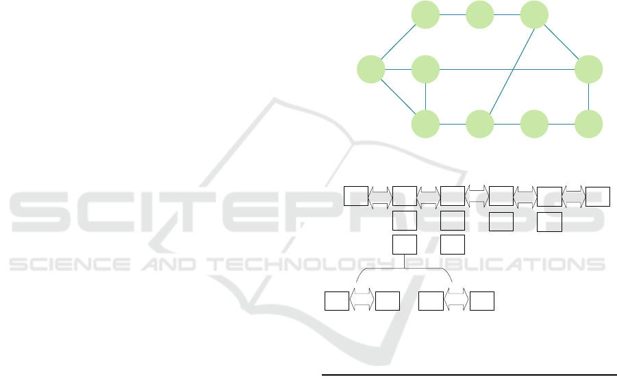
An example of layering network topology is
shown as in Figure 2. Figure 2 (a) shows the original
physical network, and Figure 2 (b) shows the
information of the layered topology. We assume that
the request client node
is the node A, and the
destination client node
is the node I. We put the
request client node A in the L.1 (V
1
is the set of
nodes in L.1) and put the nodes B, C, D which are all
directly connect with the node A in the L.2, then we
put the nodes E, F, I which are directly connect with
the nodes of L.2 in the L.3. In our network layering
strategy, the nodes in the next layer must directly
connect with the nodes except for the destination
client node I in the last layer. Thus, G, H, J directly
connect with the nodes in the L.3, while J connects
with the destination client node I, it can’t be put in
the next layer L.4. We only put the node G and H
into the L.4. And I, J connect with G, H which are in
the L.4, so we put node I, J in the layer L.5 (all
nodes except for the destination client node I can be
belong to only one layer) and I connect with the
node J, we put it in the L.6. The overall network
layering process finishes when all of the nodes in G
are included into corresponding layers. All nodes
except for the destination client node I can be in
only one layer. For each layer, we need to layer the
inner layer network topology, and get the inner
information
about the L.X. In the example, only
the L.2 has the inner layer and it includes two layers.
So the Algorithm 2 layers L.2 composed by node B,
C and D, and then gets the corresponding
information of inner layers. As
shown in the
Figure 2 (b), for each layer X<= L
MAX
and each node
N
i
∈V.X should be set as the request client node
and let N
a
= , then we get the inner layer
information about all the nodes. In
, the
and
both are 2, while
is 1. As a result, the
physical network is layered into six layers. The
source client node
is only in the layer L.1 and the
destination client node N
a
is in the layers L.3, L.5
and L.6. It means that there are at last three paths to
connect
with
. We use
to denote the length
of the path (the length of the three paths are
respective three, five and six), which equates the
number of the VNFs that the path can hold,
meanwhile the notation L
S
is the length of SFC that
denotes the number of VNFs in a SFC.
A
B
C
D F
E
H J
I
G
(a) The physical network
L.1; V
1
L.3; V
3
L.2; V
2
L.4; V
4
L.5; V
5
L.6; V
6
V
(2,2)
C
V
(2,2)
D
V
(2,1)
D
B
C
D
E
F
I
G
H
I
J
I
A
D C
V
(2,1)
C
C D
(b) The layered topology
Figure 2: Example for layering a physical network.
Algorithm 2:Physical network layering
Input: (1) Substrate network G;
(2)
; (3)
.
Output:
;
1:
;
= L.1;
2:for
;
; do
3: for each
; do
4: if
&&
5:
;
6: else
&&
&&
=
7:
;
8: end if
9: end for
10:
++;
11:end for
12:for L.X =<
; do
An Efficient Approach for Service Function Chain Deployment
615

13: for
; do
14:
;
15:
=
.1;
16: for
; do
17: if
&&
&&
18:
;
19: end if
20:
++;
21: end for
22: end for
23:end for
24:return
Algorithm 3 focuses on evaluating the nodes and
choosing the most suitable node to host
corresponding VNF. After layering the physical
network, Algorithm 3 can directly judge that whether
the physical network can meet the requirement of
SFC request. When the sum of all the inner layers
and the maximal layer
of the destination client
node
are still smaller than the length of SFC
(denoted as
), the physical network is hard to meet
the user’s demand. For example, when we need to
deploy a SFC request into the physical network
shown in Figure 2 (a), the clients respectively are
located at the node A and the node I. The maximum
layer
is 6, and the layer L.2 has the inner layer
and there is a layer in the inner layer, the total
number of layering network is 7. So the physical
network can meet the requirement of SFC request
whose length is no more than 7. If the length of the
SFC request is longer than 7, it is heavy for the
network. Although it can find ways to place the SFC
request, but it may consume more time and
bandwidth resources since the length of SFC
is
too long for the physical network. Our proposed
Algorithm 3 can solve the problem by searching the
nodes in the opposite direction. To address this
issue, Algorithm 3 usually find the next node in the
next layer V
N
rather than in the upper layer V
U
and
then it can directly increases the maximum length of
path (denoted as
). Considering an extreme
situation, the client is in the
without the next
layer, our algorithm allows to firstly find a node in
the upper layer
and then layers the physical
network again. And then, the found node just now
isn’t in the
.
Finally, we need to choose the suitable nodes
from the layered network to deploy the VNFs.
Algorithm 3 follows the strategy mentioned above to
find the path from
to
.
The algorithm chooses
the nodes among the layers according to Equation
(7). The chosen node must directly connect with the
node in the next layer V
N
.
,
si ri se re s r
si se s
B B B B C C
Min
B B C
(7)
We define to measure a node’s justifiability for
the SFC request. Where
means the available
bandwidth of all links which connects the nodes in
the next layer
, and
represents the requested
bandwidth for the communication between this VNF
and the next VNF.
denotes the available
bandwidth of the path which connects the nodes in
, and
represents the request bandwidth
between this VNF and the last VNF.
represents
the available computing resources in node and
represents the requested computing resources of the
corresponding VNF. And then, we choose the node
which has the minimum value of.
Algorithm 3: Node evaluation
Input:(1)
;
(2) SFC request;
(3) X:
;
(4) bool: direction;
Output:
: the node has minimum ;
1:Temp =
2: if (direction)
3: int i = 1;
4: else
5: int i = -1;
6: for
; do
7: if
;
8: if
>
&&
>
&&
>
;
9: Compute based on Equa.(2);
10: if < Temp
11: Temp = ;
12:
=
;
13: end if
14: end if
15: end if
16:end for
17:return
.
4 SIMULATION RESULT AND
ANALYSIS
With the increasing of SFC requests, to deploy SFC
requests in a static network will become more and
more challenge, thus it’s important to improve the
scalability of network. Network-aware scaling
strategy is important for extending the network
rather than changing the network blindly. Here, we
define the perceiving information
of network G
as in Equation (8).
ICEIS 2018 - 20th International Conference on Enterprise Information Systems
616
1
()
MAX
iX
L
S
s si se
X N V
G C B B
(8)
Our SFCD-LEMB algorithm layers the network
and finds the “weak” layer (i.e., the layer has
minimum resource) and analyses its inner
information and then gets the “weak” nodes or links
which influence the network’s capacity. Then the
SFCD-LEMB algorithm extends corresponding
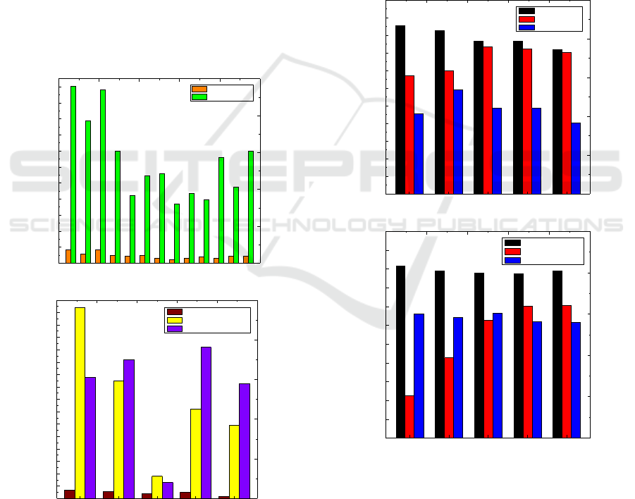
resources to make the network more robust. Figure 3
shows the results for running the SFCD-LEMB
algorithm in a small scale network. Figure 3 (a)
shows the information of whole network. Obviously,
L.8 limits the overall capacity of the network and
thus influences the users’ experience. Whereas
Figure 3 (b) gives the information about the nodes in
L.8. Node 67 has minimum bandwidth and node 72
has minimum compute resources. Both of them are
the “weak points” of the network and increasing the
corresponding resources will enhance the capacity of
physical network.
1 2 3 4 5 6 7 8 9 10 11 12 13
0
100
200
300
400
500
600
700
800
900
1000
1100
Capacity (Units)
# Layer
Node Capacity
Link Capacity
(a)
61 65 67 69 72
0
10
20
30
40
50
60
70
80
90
100
110
120
130
140
150
160
Resources (Units)
# Nodes
Computing resources
Bandwidth of last layer
Bandwidth of next layer
(b)
Figure 3: Simulation results for scaling the network.
In order to evaluate the performance of our
algorithm, we introduce two algorithms which are
Closed-Loop with Critical Mapping Feedback
(CCMF) (Zilong Ye et al., 2016) and Key-VNF
Deploy First (KVDF) which firstly deploy the key
VNF for more efficiently placing the SFC to
compare with our SFCD-LEMB algorithm.
We respectively evaluate three algorithms in
small and large scale networks. Both network
topologies are generated by using GT-ITM. In the
small scale networks, there are 100 physical nodes
and about 400 links. In the large scale networks,
there are 1000 physical nodes and about 4000 links.
In the two networks, the computing resources of
each node are 10 units, and the bandwidth resources
of each link are uniformly distributed at 100~200
units. We generate SFC requests with the
varies
from 5 to 13, and under each L
S
, we randomly
generate 10000 SFC requests.
5 7 9 11 13
0
10
20
30
40
50
60
70
80
90
100
110
Acceptance Ratio (%)
Length of SFC
SFCD-LEMD
CCMF
KVDF
(a)
5 7 9 11 13
0
10
20
30
40
50
60
70
80
90
100
110
Acceptance Ratio (%)
Length of SFC
SFCD-LEMB
CCMF
KVDF
(b)
Figure 4: Acceptance ratios in small and large scale
networks.
Figure 4 shows the evaluation result about the
acceptance ratios of the compared algorithms. Figure
4 (a) and (b) respectively show the evaluation results
in small and large scale networks. We can see that
SFCD-LEMB algorithm has a higher acceptance
An Efficient Approach for Service Function Chain Deployment
617
ratio than CCMF algorithm and KVDF algorithm.
Furthermore, the SFCD-LEMB algorithm has a
relatively stable acceptance ratio in the different
scale network and different
. It’s because that the
SFCD-LEMB algorithm has a perception about the
network after layering the physical network and it
can deploy the SFC appropriately. In addition, our
SFCD-LEMB algorithm has a better performance in
the large scale network than that in small scale
network.
Figure 5 shows the evaluation results about the
running time of SFCD-LEMB, CCMF and KVDF
algorithms. Figure 5 (a) and (b) show the evaluation
result in the small scale network and the large scale
network, respectively. In the compared algorithms,
SFCD-LEMB algorithm accomplishes the
deployment in the shortest time in both small and
large scale networks. Moreover, the running time of
SFCD-LEMB algorithm increases slowly with the
growth of the value of the length of SFC (i.e.,
).
This is because that SFCD-LEMB algorithm can
more quickly find the corresponding node to deploy
VNFs and the corresponding path to deploy SFC by
using the layering information of the network.
6 8 10 12 14
0
2
4
6
8
10
12
14
16
18
20
22
24
26
28
Time (Units)
Length of SFC
SFCD-LEMB
CCMF
KVDF
(a)
5 7 9 11 13
0
40
80
120
160
200
240
280
320
360
400
440
480
520
Time (Units)
Length of SFC
SFCD-LEMB
CCMF
KVDF
(b)
Figure 5: Running time of small and large scale networks.
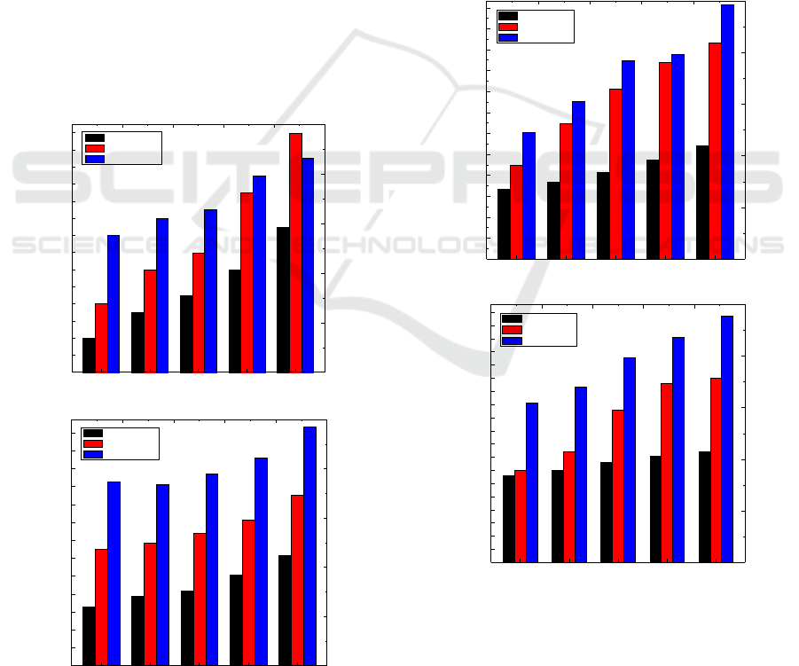
Figure 6 (a) and (b) show the evaluation results
about the bandwidth consumptions in small scale
network and large scale network, respectively. From
Figure 6 we can see that the SFCD -LEMB
algorithm can deploy SFC with less bandwidth
consumption whereas the CCMF algorithm and the
KVDF algorithm need to consume more bandwidth
to deploy the same SFC requests. With the
increasing of
and the network’s scale, the SFCD-
LEMB still has an outstanding performance in
saving the bandwidth resource. This is because that
the SFCD-LEMB algorithm can get the layering
information of the network nodes and links through
layering the physical network, which is one of the
main contributions of SFCD-LEMB. Due to layering
the physical network, the SFCD-LEMB algorithm
can save much bandwidth consumption while
increasing the capacity and scale of network.
5 7 9 11 13
0
30
60
90
120
150
180
210
240
270
300
330
360
Bandwith (Units)
Length of SFC
SFCD-LEMB
CCMF
KVDF
(a)
5 7 9 11 13
0
50
100
150
200
250
300
350
400
450
500
550
600
650
700
750
800
850
900
950
Bandwith (Units)
Length of SFC
SFCD-LEMB
CCMF
KVDF
(b)
Figure 6: Bandwidth consumption in different networks.
ICEIS 2018 - 20th International Conference on Enterprise Information Systems
618

5 CONCLUSIONS
In this paper, we study the problem of efficiently
deploying service function chains. To solve this
problem, we propose an efficient algorithm, SFCD-
LEMB, which achieves the layering information of
the network nodes and links by layering the physical
network and evaluates the physical network nodes
and then chooses the most suitable node to host the
VNFs of SFC. Simulation results show that our
proposed algorithm has good performance on
acceptance ratio, running time and bandwidth
consumption for provisioning SFC requests. In
addition, we can extend the network to satisfy the
increasing demand according to the layering
information.
ACKNOWLEDGEMENT
This research was partially supported by the National
Natural Science Foundation of China (61571098),
Fundamental Research Funds for the Central
Universities (ZYGX2016J217).
REFERENCES
Min Sang Yoon, Ahmed E. Kamal, 2016. NFV Resource
Allocation using Mixed Queuing Network Model. In
IEEE Global Communications Conference. 1-7.
Minh-Tuan Thai, Yang-Dar Lin, Yuan-Cheng Lai, 2016.
A Joint and Server Load Balancing Algorithm for
Chaining Virtualized Network Functions. In IEEE
International Conference on Communications. 1-6.
Rami Cohen, Liane Lewin-Eytan, Joseph (Seffi) Naor and
Danny Raz, 2015. Near Optimal Placement of Virtual
Network Functions. In IEEE Conference on
Computer Communications. 1346-1354.
Juliver Gil Herrera and Juan Felipe Botero, 2016.
Resource Allocation in NFV: A Comprehensive
Survey. In IEEE Transactions on Network and
Service Management. 13(3), 518-532.
Sevil Mehraghdam, Matthias Keller, Holger Karl, 2014.
Specifying and Placing Chains of Virtual Network
Functions. In IEEE 3rd International Conference on
Cloud Networking. 7-13.
Carla Mouradian, Tonmoy Saha, Jagruti Sahoo, Roch
Glitho, Monique Morrow, Paul Polakos, 2015. NFV
Based Gateways for Virtualized Wireless Sensor
Networks: A Case Study. In IEEE International
Conference on Communication Workshop. 1883-
1888.
Tachun Lin, Zhili Zhou, Massimo Tornatore and
Biswanath Mukherjee, 2016. Demand-Aware
Network Function Placement. In Journal of
Lightwave Technology. 34(11), 2590-2600.
Bo Han, Vijay Gopalakrishnan, Lusheng Ji and Seungjoon
Lee, 2015. Network Function Virtualization:
Challenges and Opportunities for Innovations. In
IEEE Communications Magazine. 53(2), 90-97.
Maryam Jalalitabar, Guangchun Luo, Chenguang Kong
and Xiaojun Cao, 2016. Service Function Graph
Design and Mapping for NFV with Priority
Dependence. In IEEE Global Communications
Conference. 1-5.
Rashid Mijumbi, Joan Serrat, Juan-Luis Gorricho, Niels
Bouten, Filip De Turck, Raouf Boutaba, 2016.
Network Function Virtualization: State-of-the-art and
Research Challenges. In IEEE Communications
Surveys and Tutorials. 18(1), 236-262.
Zilong Ye, Xiaojun Cao, Jianping Wang, Hongfang Yu,
and Chunming Qiao, 2016. Joint Topology Design
and Mapping of Service Function Chains for
Efficient, Scalable, and Reliable Network Functions
Virtualization. In IEEE Network. 30(3), 81-87.
An Efficient Approach for Service Function Chain Deployment
619
