Usage Proﬁle Rating of Suitability to E-Vehicles Utilizing a Physical

Consumption Model

Florian Hertrampf, Sebastian Apel and Steffen Sp

athe

Department of Computer Science, Friedrich Schiller University Jena, Ernst-Abbe-Platz 2, Jena, Germany

Keywords:

Electricity Consumption, Electric Vehicles, Simulation of Consumption, Timeseries Analytics.

Abstract:

The project “Wohnungswirtschaftlich integrierte netzneutrale Elektromobilitat in Quartier und Region”

(WINNER) aims to integrate shared electric vehicles, smart local grids and renewable energy in tenant house-

holds. This paper focuses on how to ﬁnd the model of an electric vehicle (consumption, recharging, usage)

which perfectly matches the requirements of particular carsharing stations. This approach utilizes usage pro-

ﬁles of conventional combustion vehicles. Each proﬁle describes booking time and distance. Applying that

information to a rating model which simulates the driving task and charges the vehicle between usages should

be able to tell how much bookings might be handled by an electric vehicle. Within this paper, we give an

introduction to our simulation system. This covers the data model, transforming bookings into driving tasks,

and the consumption and charging model itself. Further, we validate the model by using high detailed data

captured on regular routes as well as booking sets with electric vehicles. This validation shows an average

relative error of 10 % for high detailed data from and an average relative error for booking information with

known consumptions of 5 %. Finally, we present the application of our simulation system to make a decision

based on historical booking information. This application example shows that 90% usages at some station

might be handled with electric vehicles, while others should not be replaced.

1 INTRODUCTION

Mostly stated, electric vehicles (EVs) have limited

ranges until and cause the assumption that they are not

universally applicable (Bundesministerium f

ur Bil-

dung und Forschung, 2013, S. 3). The question arises

as to when an EV will become usable for private use.

This issue is usually answered through generalized

studies in which not everyone sees themselves re-

ﬂected individually. However, the following approach

implements a simulation system which helps to rate

individual usage proﬁles. The rating weights the suit-

ability to EVs and might help to decide if a personal

vehicle usage proﬁle can also be managed by using

an EV. This simulation system utilizes a physical

consumption model which provides consumptions on

particular driving situations based on technical spec-

iﬁcations of EVs as well as current real-world data,

e. g., velocity, acceleration and gradient.

This approach is made within the research project

WINNER (Chemnitzer Siedlungsgemeinschaft eG,

2017) which aims to integrate and coordinate elec-

tromobility, the energy consumption of tenant house-

holds and the local production of electricity, e. g., by

integrating photovoltaic systems into a smart local en-

ergy grid. Within the project, EVs are used via the

carsharing approach. This EV usage leads to the re-

quest about which carsharing station should use EV

as well as which might be the best EV at a particular

carsharing station. Vehicles used within carsharing

provide perfectly documented usage proﬁles. They

have to be our primary input, next to technical speci-

ﬁcations of EV, to rate them.

Within this paper, we want to use such usage pro-

ﬁles and rate them for suitability to EV by utilizing

a physical consumption model. Further, we want to

give an example of how well this approach works.

However, we have to implement the simulation sys-

tem itself, validate the particular components. Val-

idation is done by using detailed measurement data

gathered while driving with an i-MiEV on regular

routes. In addition, our project partner Mobiltiy Cen-

ter GmbH provides us with a set of anonymized us-

age proﬁles with the EV e-Golf for further validation

of our simulation system. Finally, we used another

set of anonymized usage proﬁles, also from Mobiltiy

Center GmbH, with various conventional combustion

vehicles for ﬁnal evaluations.

446

Hertrampf, F., Apel, S. and Späthe, S.

Usage Proﬁle Rating of Suitability to E-Vehicles Utilizing a Physical Consumption Model.

DOI: 10.5220/0006774904460453

In Proceedings of the 4th International Conference on Vehicle Technology and Intelligent Transport Systems (VEHITS 2018), pages 446-453

ISBN: 978-989-758-293-6

The paper starts in Section 2 with related work

about physical and statistical consumption models

used in combination with EVs. Subsequently, in Sec-

tion 3, details of the intended rating procedure are pre-

sented. As a result of that, the required components

of our simulation systems are introduced, like data

model and consumption model. The resulting system

is validated in Section 5. Finally, we evaluate usage

proﬁles of vehicles with combustion engines in Sec-

tion 6 and discuss the results in Section 7.

2 RELATED WORK

The research area of electric vehicle simulation has

become a well known subject in the last years. Up-

coming usage of EVs improves this fact. The primary

goals of research are forecasting the available ranges

or the consumed amounts of electric energy. We can

state three principles of doing this:

1. Standard driving cycles like New European Drive

Cycle (NEDC) (Verband der Automobilindustrie,

2017)

2. Statistical analysis and artiﬁcial neural network

(ANN) (Kretzschmar et al., 2013; Gebhardt et al.,

2015; Ferreira et al., 2013)

3. Physical models of EV (Rami Abousleiman,

2015; Cedric De Cauwer, 2015; Schreiber et al.,

2014; Fetene, 2014; Zhang and Yao, 2015)

The ﬁrst mentioned variant is commonly used to

get the range the car manufacturer states. The mea-

surement occurs under standard conditions, i. e. 25

◦

or 77

◦

F and with a mileage of 11 km. Out of that

the capacity of accumulators depends on temperature.

Thus, this standard driving cycle does not cover pos-

sible range decreases caused by lower ambient tem-

peratures.

Statistical analysis can be done if there are enough

data to examine, e. g. when using ANNs or regression

models. If this is available, we could search relations

between timestamps, trafﬁc, driver, weather and elec-

tricity consumption. Examples of approaches like this

can be found in research projects, e. g., eTelematik

(Kretzschmar et al., 2013) and SCL (Gebhardt et al.,

2015) as well within the Electric Vehicle Assistant de-

scribed in (Ferreira et al., 2013). Especially if a ﬂeet

of vehicles is available, we can think of this approach.

Taking up the position of a physicist, we could

develop an EV model. Using the vehicle parameters

like mass, front face or roll friction you can calculate

the forces affecting the vehicle. The corresponding

equations result in needed power and energy amount.

Rami Abousleiman (Rami Abousleiman, 2015) fol-

lows this idea. Five different routes are used to vali-

date the physical model. The consumption of electric-

ity is measured and compared to the simulated one.

Cedric De Cauwer (Cedric De Cauwer, 2015) not

only uses a physical model, a logger for Global Po-

sitioning System (GPS) coordinates and battery data

like current and voltage was used too. So very de-

tailed information is gained, and no predeﬁned tracks

are necessary. Even the recuperation of EVs can be

involved, as shown by (Zhang and Yao, 2015). They

used a speciﬁc recuperation factor for regaining en-

ergy by breaking depending on the current velocity of

the vehicle.

3 USAGE PROFILE RATING

In case of rating the suitability of an EV based on us-

ages requires specifying the possible level of detail

of such proﬁles. Within our scenario, it is necessary

to limit usage proﬁles on a set of tuples containing

start time, duration and distance to drive. This set is

sorted by starting time. The resulting end time, based

on start time and duration, should not be greater than

the starting time of the next element. Furthermore, it

is required to recharge the EV between two elements

within the sets of usages. Thus, the EV rating consid-

ers that each usage can use as much energy as it could

have until now. Additionally, if a single usage can-

not be handled, the model should use this period as

an additional recharging phase. Based on this input,

our goal is to rate the suitability of an EV. A rating,

in this case, describes how many elements of this set

of usages can be executed by using an EV. Possible

EVs might be preselected, but it is not guaranteed that

there is already a signiﬁcant amount of recorded data

for each EV-model. Based on this restriction, we can-

not easily utilize approaches like ANN or statistical

analysis. We decided to create this rating approach on

top of a physical consumption model which requires

basic car information. Information like that can be

gathered from technical speciﬁcations as well as pub-

licly available benchmark data.

The usage proﬁle rating can ﬁnally be described as

a function which takes a vehicle conﬁguration V and

a set of usage proﬁle tuples U

which are deﬁned as

start

end

,d), i. e. start time, end time and driven dis-

tance. The rating itself is deﬁned as the ratio between

usages which can be handled and usages which can

not be done because the State of Charge (charge level

of the electric vehicle) (SoC) is going to be negative.

The resulting rating function r(V,U

,...,U

) is shown

in Equation 1. It utilizes the function d(V,U

) which

Usage Proﬁle Rating of Suitability to E-Vehicles Utilizing a Physical Consumption Model

447

Usage

Prole

Consumption Charging

Vehicle Information

Rating

Simulation

Usage Splitting

Figure 1: The basic architecture of simulation system using

a usage proﬁle and vehicle information as input and outputs

rating by utilizing a consumption and charging model.

calculates the consumption within a driving task and

the function c(V,U

i−1

) which handles charging

tasks between two usages.

d : (V,U

) → 4SoC

c : (V,U

i−1

) → 4SoC

f : (V,U

i−1

) →

(

c(V,U

i−1

) + d(V,U

) |i > 0

1 − d(V,U

) |i = 0

u : (V,U

,...,U

) → { j : j =

∑

i=0

f (V,U

i−1

) ∧ m < n}

r : (V,U

,...,U

) →

|{e : e ∈ u(V,U

,...,U

) ∧ e ≥ 0}|

|u(V,U

,...,U

(1)

4 SIMULATION SYSTEM

The simulation system, as shown in Fig. 1, realizes

the already mentioned workﬂow from Section 3. De-

tails on the consumption are presented in Section 4.2

and charging calculation itself is shown in Section 4.3.

The consumption and charging model require reﬁning

the usage proﬁle into more speciﬁc tasks. Each task

can be a driving task or a charging task. A charge task

is described by time and amount of possible charging

energy. A driving task is deﬁned by a set of steps to

drive by. Each step describes a time, a velocity, the

temperature and gradient for this driving step. The

job of the splitting component within the simulation

system is to transform single usages into tasks. This

splitting strategy should be conﬁgurable to reﬂect a

different kind of situations.

4.1 Usage Splitting

Calculating consumptions based on drive tasks re-

quires detailed information on usage. In the case

of this simulation system, information should cover

tuples containing speed, duration, gradient and tem-

perature. But booking information is not that ﬁne-

grained.

The simulation system utilizes the usage splitting

component to transform initial booking information

to generate more detailed driving tasks. The follow-

ing list will show our current available strategies to

create driving tasks based on bookings.

• Uniformly.

The most simple strategy to drive. Simply drive

the booking duration with constant velocity.

• Middling.

Adds accelerations and decelerations processes

within this chain of route tasks. The number of

accelerations and decelerations can be conﬁgured.

• CommonMiddling.

Utilizes Middling and adds calculated mean ve-

locities based on driven distances. E. g., drive

50km with 40

/h and everything further with

/h. Each part can be conﬁgured with a dis-

tance to drive, a mean velocity to handle as well

as the amount of accelerations and decelerations.

4.2 Consumption Model

For calculating and comparing energy consumptions,

we use the equations for kinetic, potential and rota-

tional energy. The energy budget of a single vehicle

may compare well to the values of others. But the en-

ergy loss caused by friction between tires and surface

or car body and surrounding air needs to be modelled

as well. This can be done by using the resulting fric-

tion forces and multiplying them by the actual veloc-

ity. So we gain the currently needed power to keep a

speciﬁc velocity. Multiplying by the necessary time

we calculate the consumed energy. The following list

gives a short overview.

• Air friction F

air

• Roll friction of tires F

roll

• Gradient of surface F

grad

• Inertia of vehicle F

• Wheel rotation caused by inertia F

wheelrot

• Engine’s torque moving the vehicle F

The modelling of the formerly mentioned aspects

referring to consumption needs some vehicle speciﬁc

parameters. We need the mass of the car, the mass

of the wheels (moment of inertia required), the mea-

surements and drag coefﬁcient (front face calculation

for air drag) and the capacity of the accumulator. Out

of that, we need the temperature of the environment

and the gradient of the terrain. The latter informa-

tion is used to calculate the fractions of the gravity

force, which correspond with the tire friction (orthog-

onal force to the terrain) or the grade resistance (par-

allel to the terrain). The temperature is essential for

the capacity of the accumulator and affects the range.

VEHITS 2018 - 4th International Conference on Vehicle Technology and Intelligent Transport Systems

448

There are some problems with the formerly men-

tioned values. Getting the measurements etc. does not

state a problem, but the dependency of capacity on the

temperature may not linear. Furthermore, the mass of

the engine and its rotating parts cannot be found easily

in technical speciﬁcations of EV published by manu-

facturers. Furthermore, if we consider acceleration

phases, the velocity is changing as well as the acting

forces. Thus, we calculated the integrals of the forces

multiplied by travelled distances to estimate the pro-

duced and consumed energies. The results are multi-

plied by the matching distortion factor for energy con-

sumption or recuperation (Listing 2, (Hertrampf et al.,

2018)).

air

+ E

roll

+ E

pot

+ E

kin

+ E

rotwheel

+ E

rotengine

(

∆E

total

· consumptionfactor |∆E

total

> 0

∆E

total

· recuperationfactor |∆E

total

< 0

(2)

Finally, we use a factor to tare our model. The fac-

tor describes how much kilometres the evaluated car

may travel without recharging in relation to our sim-

ulation result. In fact, this factor is multiplied by the

consumed energy. For further information, a techni-

cal report is available under (Hertrampf et al., 2018).

We had no chance of validating the technical details

like air resistance coefﬁcient or roll friction of the

EV itself. Only manufacturer’s information or gen-

eral physical information was used, e. g. roll friction

of standard tires.

4.3 Charging Model

The energy consumption can be modelled by using

an efﬁciency factor within our stepwise simulation.

In contrast, the charge task is not mapped onto steps.

This is caused by the lack of charging information on

the EVs. We would not have been able to check our

model according to the considered vehicles. Fortu-

nately, there is some research on this term. Moham-

mad Chahgrkhgard (Charkhgard and Farrokhi, 2010)

states a root-shaped proﬁle for the SoC over time. Ac-

cording to this result and empirical values, we use a

double-linear charging proﬁle. Up to a threshold of

reﬁlled capacity the model charges with a high ef-

ﬁciency, afterwards, the efﬁciency is reduced. This

simple charging model accounts for the fact, that ve-

hicle manufacturers often state charging times up to

80% and the remaining time up to 100%.

4.4 Reality Distortion Factor

One factor can modify the consumption model of Sec-

tion 4.2. This factor might be used to overcome the

gap between the physical consumption and the real

consumption of an EV. However, the goal of this

paper is to rate usage proﬁles of suitability to EV

utilizing. Further, this rating is done without hav-

ing recorded driving data. To solve the problem of

missing driving data, the idea is to get this factor by

using available information driving results and com-

pare them to consumptions made by our consumption

model.

The NEDC (Verband der Automobilindustrie,

2017; Nations, 1995) is a standardized driving cycle

with a distance d

NEDC

of 11022 m which takes 1180 s

to drive. Manufacturers mostly provide results as con-

sumption per kilometre or driving range in kilometres.

The NEDC cycle measures the energy consumed after

driving the cycle two times on a roller dynamometer.

This measurement is done after a full discharge and

recharge of the vehicle.

Within our simulation system, we use this cycle

to get the energy consumption ∆E

Model

based on our

model as it would be with a speciﬁc car mass, front

face and air drag coefﬁcient. Afterwards, we calculate

the max range of this consumption and the vehicle ca-

pacity C as the NEDC does it and compare this result

to the NEDC-range R

NEDC

a vehicle should have:

RDF ·

∆E

Model

NEDC

The resulting ratio is used as our reality distortion

factor (RDF). This factor should compensate speciﬁc

efﬁciencies of the EV as well as various loss factors

between the point of measurement used by the NEDC

and the point of the simulation. The equipment is

placed between vehicle charger and main socket to

measure consumptions afterwards. Our consump-

tion model calculates energies required to change the

moving state and position of the EV.

Getting the RDF has to be an iterative process.

The NEDC causes this. We do not know the technical

efﬁciency of an EV, which handles the driving cycle.

So we assume at ﬁrst an RDF of 1, that means, we

estimate a model consumption equal to the real con-

sumption. After driving the NEDC, we compare the

manufacturer’s given range and the simulated and cal-

culated range. Depending on this comparison we gain

a new value for the distortion. Using this number, we

rerun the simulation and use the next distortion value

obtained in this way. The steps are repeated up to

such time as we get no difference between start dis-

tortion and end distortion. Finally, we get the vehicle

speciﬁc RDF that we can use for the further evalua-

tion of usage proﬁles. Fig. 2 shows the progress of

the factor calculation. You can see, that 10 to 20 cy-

cles are enough to get a value changing no longer. The

Usage Proﬁle Rating of Suitability to E-Vehicles Utilizing a Physical Consumption Model

449

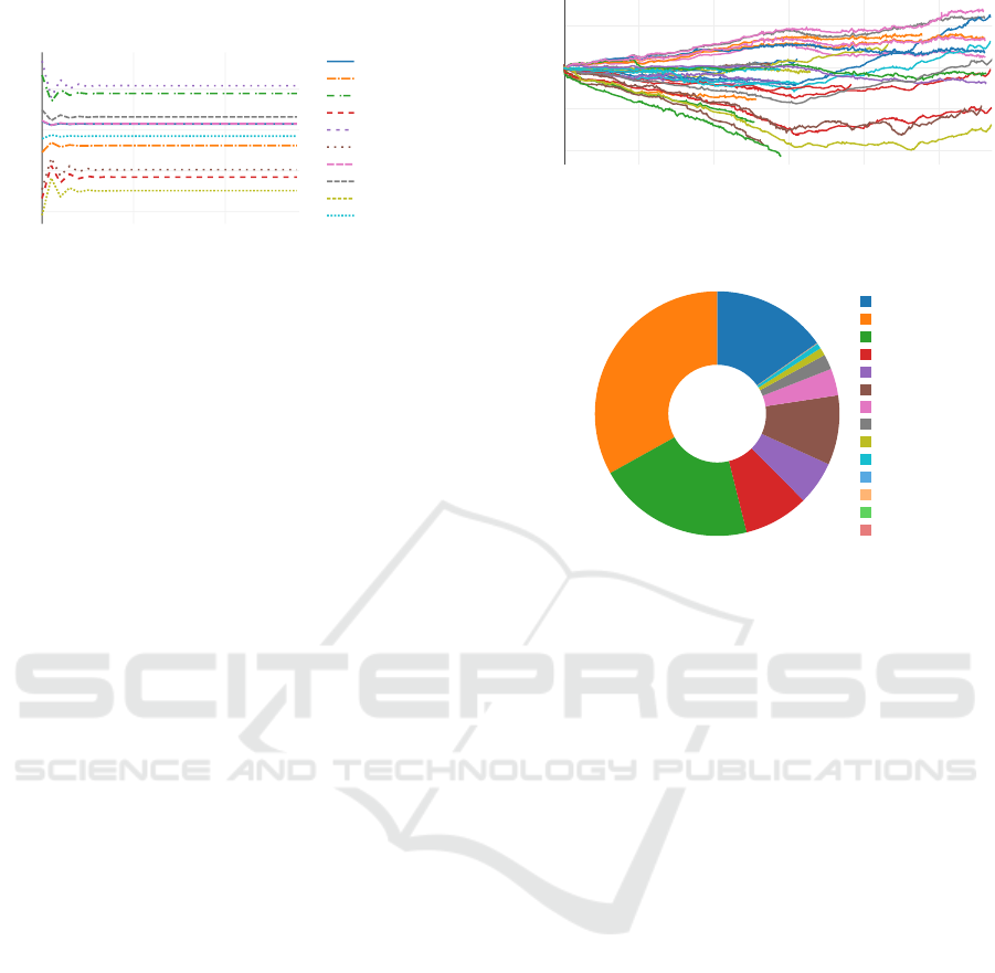
i-MiEV reaches a value of approx. 1.09 for example.

0 10 20

0.8

0.9

1.1

Cycles

Reality Distortion Factor

Kangoo Z.E.

eNV200

i3 (94 Ah)

eup!

ZOE 22

eGolf

i3 (60 Ah)

ZOE 41

fortwo electric drive

iMiEV

Figure 2: Distortion factor plotted over number of repetitive

calculations.

5 VALIDATION

We have to show the usefulness of our model. For this

approach, we used data from tracks collected in 2013.

The tracks run from Jena to Weimar and back as well

as from Jena to Golmsdorf and back. In this section,

we give a short description of this information and

identify problems.

5.1 Speciﬁc Validation

The validation of our physical model is done by us-

ing data from a Mitsubishi i-MiEV. We use the OBD2

Port to access CAN-Bus data, i. e. the current veloc-

ity, the measured state of charge of the battery and

the needed current and voltage at a speciﬁc time. Ad-

ditionally, we have added the current GPS position.

Using the position data we called an elevation web

service (Google, 2017) to gain information on the cur-

rent gradient. The time resolution is one second. At

this point, we must state, that the quality of data is

not perfect. If we compare the velocity calculated by

the GPS locations and the velocity measured recorded

from the OBD2 Port we get differences. Furthermore,

there is a mismatch between the measured SoC and

the iterative summed up energy. So we have to choose

one single data source, or we have to interpolate be-

tween various values. We do not consider current

weather conditions or driving characteristics of spe-

ciﬁc car drivers. This validation utilizes the already

mentioned RDF.

Situations, like driving uphill, while decelerating

or driver speciﬁc behaviour, cause problems and an

error of energy consumption forecast. Driving uphill

or downhill with a large gradient is not modelled per-

fectly. For lower gradients, the prognosis gets better.

Finally, we want to present the overall error for

the i-MiEV on various tracks. Fig. 3 shows that we

get results differing from the measured consumptions

by an amount of 10 %. The error is not increasing

0 10k 20k 30k 40k 50k

0.9

0.95

1.05

Distance in m

Relative Error

Figure 3: Evolution of errors on various tracks depending

on track distance (vehicle i-MiEV).

15.2%

33.1%

20.8%

8.57%

5.77%

9.19%

100

150

200

300

400

500

1000

other

Figure 4: Grouped distances in usage proﬁles (15.2 % is

smallest category 10, other categories anti-clockwise).

constantly. Some tracks show an increasing and de-

creasing evolution. We assume that the weather con-

ditions and the driver behaviour are responsible for

this irregular process in addition to the insufﬁciencies

mentioned above. Considering these inaccuracies, the

error has got a small value.

5.2 Splitting

Until now, we have validated that our consumption

model calculates consumptions which are compara-

ble to measured ones. We want to use this validated

part of our simulation system and take a closer look at

the splitting component. As mentioned, this splitting

is used to get an approximated list of driving tasks

based on a usage proﬁle U. This proﬁle is a tuple of

distance, start and end time deﬁned as (t

start

end

,d).

Our validation is done by using real usage proﬁles

from EV bookings. Those bookings contain the start

and end SoC also. Thus, we know how much energy

is used by this booking. However, these information

does not include details about charging processes.

Fig. 4 visualizes more than 4.300 usages grouped

by distances done with an E-Golf which has a range of

190km measured by NEDC. As shown, most usages

are below 100 km. We decided to drop usages with

unrealistic consumptions, i. e. consumptions per kilo-

metre lower than 0.5 % and higher than 1.5 %. This

drops approx. 350 usage proﬁles and ﬁnally removes

such ones, which include recharging tasks. These

VEHITS 2018 - 4th International Conference on Vehicle Technology and Intelligent Transport Systems

450

20k 40k 60k 80k 100k 120k

Distance in m

Relative Error in %

Figure 5: Average relative error per distance with ﬁnally

conﬁgurated CommonMiddling splitting strategy.

cannot be validated.

Making use of the splitting strategy Uniformly

(see Section 4.1 for an overview of strategies) results

in an average error of 197 %. The more distance a

usage proﬁle handles, the lower the error will be. Uti-

lizing middling strategy with acceleration and decel-

eration phase, called cycle, with 60 s, 30 s and 10 s

results in a slightly improved average error ranging

from 172 % to 51 %. However, these strategy indi-

cates better errors in particular distances as well as

much too low velocity values. Thus, we have used

the CommonMiddling strategy conﬁgured with 50 km

at 40

/h and everything further at 80

/h. The ﬁrst

50km uses 5s cycles and the remaining distance uses

60s cycles. This strategy results in an average error of

68%. Further, analyses show hot spots in various dis-

tances. Thus, we optimized the conﬁguration of our

CommonMiddling strategy with ﬁve states. They are

shown ascending in the following list. The resulting

average error is 5 % and is visualized in Fig. 5.

1 Up to 10 km at 25

/h with 5s cycles

2 Up to 30 km at 32

/h with 15s cycles

3 Up to 60 km at 70

/h with 45s cycles

4 Up to 90 km at 70

/h with 360 s cycles

5 Up to ∞km at 70

/h with 1000 s cycles

5.3 Usage Proﬁle Rating

Finally, after validating consumption model and us-

age proﬁle splitting, we like to take a closer look at the

usage proﬁle of a dataset where we know that EV uses

it. Fig. 6 visualizes the same dataset as used in Sec-

tion 5.2 splitted according to used vehicles. The ﬁnal

rating is done as introduced in Section 3. This valida-

tion intends to check if this data produces ratings at

nearly 100 %. The ﬁgure shows that the implemented

simulation system creates a rating of an already sub-

stituted EV at an average of 97.4 %.

Car#1 Car#2 Car#3 Car#4 Car#5 Car#6 Car#7 Car#8 Car#9

Suitability in %

Figure 6: Usage proﬁle rating of an EV.

20%

25.5%

11.7%

6.51%

4.9%

7.26%

4.91%

5.32%

5.95%

3.22%

100

150

200

300

400

500

1000

other

Figure 7: Grouped distances of usage proﬁles of combus-

tion vehicles (20 % is smallest category 10, other categories

anti-clockwise).

6 EVALUATION

After showing the usefulness of our model, we want

to consider some more vehicles. The usage data of

conventional combustion vehicles of a car sharing ser-

vice were used to create usage proﬁles. Our aim is to

show, which of these proﬁles could be handled by an

EV. First, we take a look at the usage proﬁles of the

combustion vehicles.

As you can see in Fig. 7 the distances mentioned

above of EV bookings are applicable for conventional

cars too. There is an amount of approx. 18 % of tracks

that are longer than 100 km. So, we expected a good

rating result for the EVs during our research. The us-

ages of them and conventional vehicles are similar in

general.

We used the formerly mentioned rating index

(Section 3) to evaluate the possibility of replacing

combustion vehicles with EV. In Fig. 8 you can see

the rating index in percent for various EV. The rating

is calculated for many combustion vehicles (1 to 49).

The indexes 21 to 27 show a low suitability value.

This might be caused by many long-distance tracks,

which had to be handled by the cars. In contrast, the

vehicle index 35 shows a high rating of 95%. This car

could have been replaced by an EV, i. e. there were

many shorter tracks to drive. An interesting case can

be found referring to car 36. We can see, that some

EV got a rating of approx. 50%, some others of ap-

prox. 90%.

Usage Proﬁle Rating of Suitability to E-Vehicles Utilizing a Physical Consumption Model

451

Kangoo Z.E.

e-NV200

i3 (94 Ah)

e-up!

ZOE 22

e-Golf

i3 (60 Ah)

ZOE 41

fortwo elect. drive

i-MiEV

Car#1

Car#2

Car#3

Car#4

Car#5

Car#6

Car#7

Car#8

Car#9

Car#10

Car#11

Car#12

Car#13

Car#14

Car#15

Car#16

Car#17

Car#18

Car#19

Car#20

Car#21

Car#22

Car#23

Car#24

Car#25

Car#26

Car#27

Car#28

Car#29

Car#30

Car#31

Car#32

Car#33

Car#34

Car#35

Car#36

Car#37

Car#38

Car#39

Car#40

Car#41

Car#42

Car#43

Car#44

Car#45

Car#46

Car#47

Car#48

Car#49

100

Suitability in %

Figure 8: Suitability factor for various EV.

All in all, we can state, that over 50 % of the

tracks driven by conventional vehicles could have

been driven by EV too. There are some distances

electric driven cars cannot handle, but it depends on

the type of EV. The capacity of the accumulator may

be a primary factor. The ZOE 41 has got the accumu-

lator with the highest capacity and reaches the best

suitability values (Fig. 8).

7 DISCUSSION

Even if we got simulated energy consumptions

matching measurement values (Fig. 3 and Fig. 6),

there are some problems although. We used the

NEDC to get RDFs for our considered EVs. At this

point, we are simulating the consumptions within the

car, not the energy we have to recharge after driving

the tasks of the cycle. This way of proceeding results

in systematic errors, which impact all the following

steps. The process of measurement of the NEDC does

not happen within the car; it only evaluates supplied

electric energy.

Another problem is caused by the external inﬂu-

ences of a driving task. At now, we do not consider

weather conditions like rain or wind. Watching these

factors, we get higher energy consumptions if there is

a headwind or if we have to use the wipers. Especially

the lights of the car are not only turned on during the

nighttime period. The modelling of the recuperation

while driving uphill or downhill is not easy because

we would have to know if the EV is recuperating or

not. But this often depends on the state of the throttle

pedal, not the velocity of the car or other macroscopic

measurement values.

The aforementioned sources of errors refer to vari-

ous driven tracks. The longer the distance a car drives,

the harder it gets to model recharging and driving. On

short tracks, there are not that many possibilities of

taking breaks for recharging. The behaviour of the

driver is tough to estimate, referring to conﬁgurated

breaks and accelerations. While working, we found

tracks of equal length which were driven by a speciﬁc

energy amount and the half of this value. Guessing

the energy economy causes errors.

A very system speciﬁc problem lies in the “Com-

monMiddling” (section 4.1). We got the strategy in

Section 5.2 by try and error. It was calibrated using

a vehicle type with about 4.000 usages. But we are

not sure if this strategy is vehicle-speciﬁc or a more

generic approach. The values reﬂect a plausible driver

behaviour, but we were not able to check them against

other vehicle models. Out of that, we did not con-

sider recharging during a driving task. Our model

only recharges between two tasks. The long-distance

tracks are not well evaluated in this way. Such tasks

need recharging by the driver, and so they get under-

valued.

As mentioned before, there are problems of mod-

elling driving uphill or downhill. The reached error

level will be hard to underbid. If we correct the model

referring to higher gradients, we get worse results for

lower ones. The physical model forces us to keep

the physical plausibility, i. e. adding correction terms,

maybe depending on time, must have a physical justi-

ﬁcation.

Although, we reach a high precision level, espe-

cially if we think of the non-existent, precise track

data for each considered vehicle.

8 CONCLUSION

Our approach aimed to decide if an EV could have

overcome the usage proﬁle of a vehicle with a com-

bustion engine. We used a physical energy model

to describe the electricity consumption of EVs. Fur-

thermore, a model for splitting up usages into driv-

ing tasks was used to guess the behaviour of a driver

(driving and charging tasks) on a speciﬁc track. Fi-

nally, we simulated the driving of EVs on them and

calculated a rating that represents the possibility of

replacing the formerly used combustion vehicle by an

EV.

VEHITS 2018 - 4th International Conference on Vehicle Technology and Intelligent Transport Systems

452

We were able to show the possible precision of a

physical model in combination with a clever-guessed

user behaviour. Within the i-MiEV validation, a limit

has been reached at least if we think of the poor data

input we used. The physical model is conﬁgurable but

needs an RDFs in the end. To overcome this problem,

additional energy consumptions must be added like

lights or air conditioning system. Furthermore, other

measurements should be done so that further energy

terms can be added. Out of that, the speciﬁc consump-

tion behaviour depending on temperature and gradient

is needed. These measurements should take place for

every considered EV.

Referring to the aforementioned additional mea-

surements we have to think of the model in general.

Maybe we should not use a physical model reﬂecting

energies. Another way could be the use of average

consumption depending on manufacturer given val-

ues. With a more signiﬁcant amount of data, an artiﬁ-

cial intelligence could be used as well. Further, an ad-

vantage would be the more precise knowledge of the

behaviour of drivers. Especially people frequently us-

ing EVs are experienced in a recuperation-enhancing

driving tactic.

However, that was not the primary question within

this approach. As shown, it seems to be possible to

rate usage proﬁles by utilizing a physical consump-

tion model. Such methods have to take into consid-

eration an average relative error of approx. 10% of

the physical consumption model itself, which might

be optimized by adding more accurate measurement

data, as well as an error of approx. 5 % when guess-

ing driving tasks within our splitting component. This

application example shows that 90 % usages at some

station might be handled with electric vehicles, while

others should not be replaced.

ACKNOWLEDGEMENTS

The research project WINNER is funded by the Fed-

eral Ministry for Economic Affairs and Energy of

Germany under project number 01ME16002D. We

would like to thank especially the Mobility Center

GmbH for the provision of anonymised booking data.

REFERENCES

Bundesministerium f

ur Bildung und Forschung

(2013). Elektromobilit

at - das Auto neu denken.

https://www.bmbf.de/pub/Elektromobiltaet das Auto

neu denken.pdf; 2017-11-30.

Cedric De Cauwer, Joeri Van Mierlo, T. C. (2015). Energy

consumption prediction for electric vehicles based on

real-world data.

Charkhgard, M. and Farrokhi, M. (2010). State-of-charge

estimation for lithium-ion batteries using neural net-

works and ekf. IEEE TRANSACTIONS ON INDUS-

TRIAL ELECTRONICS, 57(12).

Chemnitzer Siedlungsgemeinschaft eG (2017). WINNER-

Projekt. http://www.winner-projekt.de; 2018-02-01.

Ferreira, J. C., Monteiro, V., and Afonso, J. L. (2013). Dy-

namic range prediction for an electric vehicle. In

2013 World Electric Vehicle Symposium and Exhibi-

tion (EVS27), pages 1–11.

Fetene, G. M. (2014). A report on energy consumption and

range of battery electric vehicles based on real-world

driving data. Technical report, Technical University

of Denmark.

Gebhardt, K., Schau, V., and Rossak, W. (2015). Applying

stochastic methods for range prediction in e-mobility.

In Innovations for Community Services (I4CS), 2015

15th International Conference on, pages 1–4.

Google (2017). Elevation api.

https://developers.google.com/maps/documentation/

elevation/intro?hl=en; 2017-11-28.

Hertrampf, F., Apel, S., Sp

athe, S., and Rossak, W.

(2018). Modelling electric vehicle consumption - a

physical approach for the i-miev. Technical Report

Math/Inf/01/18, Friedrich Schiller University.

Kretzschmar, J., Geyer, F., Sp

athe, S., and Rossak,

W. (2013). eTelematik: Prognose und

Ausf

uhrungs

uberwachung elektriﬁzierter kom-

munaler Nutzfahrzeuge. In Schau, V., Eichler, G., and

Roth, J., editors, 10. GI/KuVS-Fachgespr

ach ”Orts-

bezogene Anwendungen und Dienste”, number 10,

pages 101–108, Jena, Germany. Logos Verlag.

Nations, U. (1995). Concerning the adoption of uniform

technical prescriptions for wheeled vehicles, equip-

ment and parts which can be ﬁtted and/or be used

on wheeled vehicles and the conditions for reciprocal

recognition of approvals granted on the basis of these

prescriptions.

Rami Abousleiman, O. R. (2015). Energy consumption

model of an electric vehicle.

Schreiber, V., Wodtke, A., and Augsburg, K. (2014). Range

prediction of electric vehicles. In Shaping the future

by engineering : 58th IWK, Ilmenau Scientiﬁc Collo-

quium.

Verband der Automobilindustrie (2017).

New european driving cycle.

https://www.vda.de/en/topics/environment-and-

climate/exhaust-emissions/emissions-measurement;

2017-11-16.

Zhang, R. and Yao, E. (2015). Electric vehicles energy con-

sumption estimation with real driving condition data.

Transportation Research Part D: Transport and Envi-

ronment, 41:177 – 187.

Usage Proﬁle Rating of Suitability to E-Vehicles Utilizing a Physical Consumption Model

453