
Investigating the Use of Primes in Hashing for Volumetric Data
L
´
eonie Buckley, Jonathan Byrne and David Moloney
Movidius, Intel, Ireland
Keywords:
Hashing, SLAM, Storage, Indexing, Volumetric Data, Primes, Voxels.
Abstract:
Traditional hashing methods used to store 3D volumetric data utilise large prime numbers. The intention of
this is to achieve well-distributed hash addresses to minimise addressing collisions. Hashing is an attractive
method to store 3D volumetric data, as it provides simple method to store, index and retrieve data. However,
implementations fail to provide theoretical support as to why they utilise large primes which act to create
a hash address through randomising key values. Neither is it specified what a “large” prime is. 3D data
is inherently well-distributed as each coordinate in 3D space is already unique. It is thus investigated in this
paper whether this randomisation through the use of large primes is necessary. The history of the use of primes
for hashing 3D data is also investigated, as is whether their use has persisted due to habit rather than due to
methodical investigation.
1 INTRODUCTION
Hashing is used to map data of arbitrary size to an
addressing space, and is a popular method to store,
retrieve and delete 3D volumetric data (Teschner
et al., 2003) (Klingensmith et al., 2015) (Niener
et al., 2013) (Eitz and Lixu, 2007) (K
¨
ahler et al.,
2015). In much of the early literature discussing hash-
ing (Knott, 1975) (Knuth, 1998), the common goal
is to achieve distinct mapping addresses. However,
Knuth states that “it is theoretically impossible to de-
fine a hash function that creates truly random data
from nonrandom data in files” (Knuth, 1998). The
birthday paradox (Good, 1950) highlights the diffi-
culty in achieving distinct addresses: if a random
function is selected to map 23 keys to a table of size
365, the probability that no two keys map to the same
location is only 0.4927.
In hashing, the address calculation is generally
achieved by a randomised scrambling of key values,
with many methods using large primes to achieve
this scrambling (Teschner et al., 2003) (Klingensmith
et al., 2015) (Niener et al., 2013) (Eitz and Lixu,
2007) (K
¨
ahler et al., 2015). Hashing is an appropriate
term, as a hash is “a random jumble achieved by hash-
ing”, where hashing means to cut or to chop (Knott,
1975).
Hash coding was first described in open liter-
ature by Arnold I. Dumey in the 1950s (Knuth,
1998) (Dumey, 1956) (although the idea of hashing
appears to have been originated by H.P Luhn in an
internal IBM memorandum in January 1953). Dumey
discusses a real life example where the details of eight
machines that are sold to the public must be stored.
To ensure that the details of no two machines would
be stored at the same address, originally the six digit
identifiers of the machines were used. However, on
inspection of the identifiers, it was found that the
fourth digit of each of them was unique. It was there-
fore sufficient to store only the fourth digit as an iden-
tifier, and release the other five for other purposes.
Although this analogy is rather extreme, Dumey ex-
plains that an examination of the item description may
reveal built-in redundancy which can be used to re-
duce memory usage.
It is important to note that the choice of Hash func-
tion is dependent on the application. Some applica-
tions are focused on maintaining data integrity (i.e
minimising the number of hashing collisions), while
others are focused on execution speed (Eitz and Lixu,
2007) (speed of data retrieval). As well as minimising
hashing collisions, another consideration is to provide
a technique that allows for an ease of data insertion
and removal, which is paramount when considering
dynamic data.
A hashing algorithm should be selected so that the
addresses are uniformly distributed (Teschner et al.,
2003). An optimal solution is to provide a per-
fect hashing function, which allows the retrieval of
data in a hash table with a single query (Jaeschke,
1981) (Sprugnoli, 1977). This would provide a hash
with no addressing collisions. Intuitively, this could
304
Buckley, L., Byrne, J. and Moloney, D.
Investigating the Use of Primes in Hashing for Volumetric Data.
DOI: 10.5220/0006797803040312
In Proceedings of the 4th International Conference on Geographical Information Systems Theory, Applications and Management (GISTAM 2018), pages 304-312
ISBN: 978-989-758-294-3
Copyright
c
2019 by SCITEPRESS – Science and Technology Publications, Lda. All rights reserved

be achieved by providing a suitably large hash table.
However, this is not always practical as volumetric
data is often used in memory confined situations, such
as for SLAM (Simultaneous Location And Mapping)
on mobile and robotic platforms using real-time sen-
sors (Klingensmith et al., 2015; K
¨
ahler et al., 2015).
What is apparent however, is that 3D volumetric data
inherently possesses well distributed voxel addresses.
Referring to hashing functions mapping different
data to the same hash address, it has been stated
that “...such collisions cannot be avoided in prac-
tice” (K
¨
ahler et al., 2015). It is true that collisions
cannot be completely avoided, but it is investigated in
this paper whether certain prime values can be chosen
to reduce/minimise the number of collisions.
This paper not only compares the use of different
prime values in 3D volumetric data, but also investi-
gates whether large primes are necessary at all. The
remainder of the paper is structured as follows:
• Section 2 - Related Work
• Section 3 - Hashing Parameters
• Section 4 - Tests administered
• Section 5 - Results
2 RELATED WORK
Anyone who attempts to generate
random numbers by deterministic
means is, of course, living in a state of
sin
John von Neumann
To understand why the use of primes in the hash-
ing of 3D data has persisted, an examination of the
most important classical hashing methods is required.
These methods are explored by Knuth (Knuth, 1998)
in much detail, some of which are described below:
2.1 Division Hashing Method
For certain scenarios, it was found that basic hashing
methods can provide adequate results by providing a
simple mapping for a memory limited map. The divi-
sion method is particularly simple (Knuth, 1998):
H(K) = K%M (1)
Where K is the identifier of the data to be hashed
(or the Key), M is an arbitrary number and % is the
modulus operator. Knuth emphasises the importance
in choosing the value of M, and how this choice can
introduce bias into the results. For example, if M is
an even number, H(K) will be even when K is even,
and odd when K is odd, which would lead to substan-
tial bias. Taking this and further considerations into
account, he suggested choosing M to be a prime num-
ber such that r
k
6= ±(a%M), where k and a are small
numbers and r is the radix of the character set. Knuth
states that using these prime numbers “has been found
to be quite satisfactory in most cases”, but does not
provide results. Note that Knuth’s recommendation
of the use of primes relates only to the case specified
above.
2.2 Multi-identifier Hashing Function
The Division Hashing Method above in Section 2.1,
while effective for simple scenarios, is only of use
for data with a single identifier. For data with multi-
ple identifiers Knuth suggests utilising multiple inde-
pendent hash functions - one per identifier - and then
combining the results in some way. This idea was
first introduced by J. L. Carter and M. N. Wegman
and the equation is given below (Knuth, 1998; Carter
and Wegman, 1979):
H(K) = (h
1
(x
1
) + h
2
(x
2
) + ... + h
l
(x
l
))%N (2)
where l is number of identifiers, h
j
is an indepen-
dent hash function, x
j
is an identifier and N is the
number of addresses available. This function is espe-
cially efficient when x
j
is a single character because
a LUT (look up table) can be utilised for h
j
, which
removes the need for multiplications.
2.3 XOR Hashing Function
Many implementations (Teschner et al., 2003) (Klin-
gensmith et al., 2015) (Niener et al., 2013) (Eitz and
Lixu, 2007)(K
¨
ahler et al., 2015) (K
¨
ahler et al., 2016)
utilise an XOR hashing function to index 3D volu-
metric data into a hash table. This hash address is
retrieved using Equation (3):
hash(x, y, z) = (P
1
∗ x ⊕ P
2
∗ y ⊕ P
3
∗ z)%N (3)
where ⊕ is the XOR operation, (P
1
, P
2
, P
3
) are se-
lected prime values, x, y, z are the 3D coordinates of
the data in the volumetric structure that is to be stored
and N is the size of the hash table. None of (Teschner
et al., 2003) (Klingensmith et al., 2015) (Niener et al.,
2013) (Eitz and Lixu, 2007) (K
¨
ahler et al., 2015) clar-
ify why large primes are utilised. It is not stipulated
in (K
¨
ahler et al., 2016) that (P
1
, P
2
, P
3
), or the “hash
coefficients” be primes.
In the case of hashing for 3D volumetric data,
XOR hashing is the most commonly used, and is thus
examined in further detail.
Investigating the Use of Primes in Hashing for Volumetric Data
305
3 PARAMETERS IN XOR
HASHING
There are many parameters that influence the results
of the chosen hashing function. As discussed in sec-
tion 1, a “successful” hash function is dependent on
the application. For the purposes of this paper, the fo-
cus is on maintaining data integrity (minimising the
number of voxels that are not stored in the hash ta-
ble due to addressing collisions) while maintaining a
reasonable data footprint. Regardless of the hashing
function chosen, the following parameters can have
an impact on the results of the function.
3.1 Use of Primes
The use of primes is common in hashing func-
tions, with (Teschner et al., 2003) (Klingensmith
et al., 2015) (Niener et al., 2013) (Eitz and Lixu,
2007) (K
¨
ahler et al., 2015) all using large primes.
Knuth (Knuth, 1998) affirms that the first mention
of using primes for hashing is by Dumey (Dumey,
1956) in 1956, where taking the remainder of divid-
ing by a prime is discussed as a method of map-
ping data to addresses in a hash table. Dumey
states: “ ...divide this number by a number
slightly less than the number of addressable locations
(the writer prefers the nearest prime)” indicating that
the choice to use primes is a personal preference.
Many factors must to be taken into considera-
tion when choosing constant/prime values in hashing
functions (Knuth, 1998). As discussed in Section 2.1,
Knuth found certain primes to be adequate when us-
ing the Division Hashing Method in Equation (1),
but does not provide a blanket endorsement for using
primes. Why the use of primes in hashing for 3D vol-
umetric data persists may be understood with the help
of a quote from John von Neumann: “Young man, in
mathematics you don’t understand things. You just
get used to them.”
3.2 Hash Table Size
The size of the hash table relates to how many hash
table addresses exist. The size of the hash table is of
importance for a number of reasons. As discussed in
Section 2.1, when the hash address is a modulus of
the hash table size, the choice of hash table size can
introduce biases. However, the focus of this paper is
to investigate the influence of using primes in hashing,
so the impact of altering the size of the hash table is
not investigated at present.
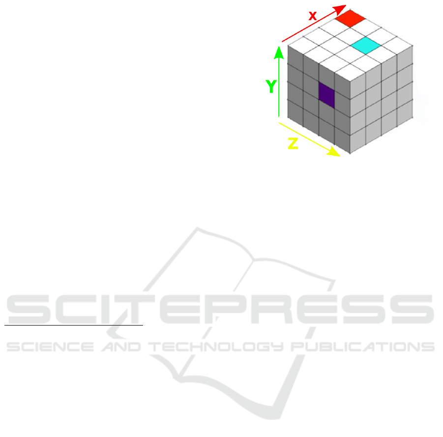
Figure 1: 4x4x4 voxel block.
3.3 Hash Table Entry Size
When H.P. Luhn first suggested hashing, he stressed
the advantage of using hash table entries that store
more than one element, as this reduces the number
of external searches required to find the correct en-
try (Knuth, 1998). The hash table entry size equates
to the number of voxels (and any other identifying
data) that can be stored in a single hash table en-
try. The blocks sizes used in other implementa-
tions vary, with some not disclosing the size (Mirtich,
1997) (Teschner et al., 2003), and others using sizes
of up to 512 voxels (8
3
) (K
¨
ahler et al., 2016) (K
¨
ahler
et al., 2015). This paper represents 64 voxels (4
3
) per
hash entry, this number is variable.
A reason for not wanting to represent a large num-
ber of voxels per hash entry is due to the sparse nature
of much 3D data - the Dublin City Dataset (Laefer
et al., 2015) was found to have an average occupancy
of 1.36% (98.74% sparse), but with a large distribu-
tion of voxels. This is similar to the typical 93% spar-
sity found in the scenes examined in (Klingensmith
et al., 2015). Representing 64 voxels per entry was
found to be adequate, as if noise is present in the form
of outliers, only a single entry would be allocated for
that noise. The larger the hash entry, the more mem-
ory will be allocated to noisy voxels.
These 64 voxels represent a 4
3
block, like the
one shown in Figure 1. When it is determined that
a voxel is occupied and must be added to the hash
table, it is first determined which block it belongs
to. In a 64
3
voxel environment, there are 16
3
4
3
blocks. The identifier of the block is taken as the
coordinates of the corner node of the block (i.e. the
red voxel in Figure 1), discretised with respect to the
size of the blocks. This is similar other implementa-
tions (Teschner et al., 2003) (Mirtich, 1997) (K
¨
ahler
et al., 2015) and (K
¨
ahler et al., 2016).
GISTAM 2018 - 4th International Conference on Geographical Information Systems Theory, Applications and Management
306

4 COMPARISON OF PRIME
VALUES FOR HASHING
To adequately determine whether large primes are
required to minimise addressing collisions, various
tests were administered on two datasets, the Stanford
Bunny (Turk and Levoy, 2005) and the Liffey Tile
from the Dublin City Dataset (Laefer et al., 2015).
Parameters for the Stanford Bunny and the Liffey tile
are shown in Table 1.
Further tests were then administered on larger, real
world datasets which are detailed in Appendix A.
Table 1: Parameters for the Stanford Bunny and the Dublin
City Dataset Liffey Tile.
Bunny Liffey Tile
Resolution 64
3
256
3
No occupied voxels 11070 234131
% Occupancy 4.2% 1.4%
Max x 63 255
Max y 62 255
Max z 49 153
Hash Table Size (No. Entries) 2040 128000
Hash Table Size (Bytes) 32kB 2MB
The following tests were carried out on the Stan-
ford Bunny and the Liffey Tile:
• Comparison of Prime Values for XOR Hashing
• Comparison of the Ordering of Prime Values for
XOR Hashing
• Comparison of Non Prime Values for XOR Hash-
ing
• Determination of the influence of the choice of
constant values on the distribution of addressing
collisions
Upon completion of the above tests, the following
were then administered on the larger, real world
datasets:
• Determination of whether “Optimum values” ex-
ist for XOR Hashing
The following actions/events occur when testing
various primes for XOR Hashing on the datasets pre-
viously mentioned:
• Insertion. Insertions into the Hash table are very
simple to perform. Once it is determined that a
voxel is occupied and should be inserted into the
hash table, the hash address of the voxel block
that the voxel belongs to is calculated using Equa-
tion 3. If an addressing collision does not occur,
the bit corresponding to that voxel in the hash en-
try is set to one. If an addressing collisions occurs
the voxel cannot be set. Dealing with collisions is
discussed below.
• Collisions. While (Teschner et al., 2003) dis-
cusses the problem of mapping different data to
the same hash address, and suggests increasing
how many voxels are represented in each hash
entry in an attempt to reduce collisions, it is not
discussed how to deal with these collisions when
they do occur. There are very simple methods in
use to deal with these collisions. (Niener et al.,
2013) deals with collisions through storing the
data to be inserted in the next available sequen-
tial entry. A.D Lin, inspired by Luhn’s early
work (Knuth, 1998), suggested a technique which
could accommodate collisions using “degenera-
tive addresses”. For example, if a collision occurs
in entry 2748, the voxels would be placed in en-
try 274, from which overflows would be placed in
entry 27 and so on.
This paper does not implement collision resolu-
tion, as the benchmarking of different prime val-
ues is concerned with the percentage of address-
ing collisions. Resolving these collisions intro-
duces additional overheads, so it is thus preferable
to invest effort into reducing the initial number of
collisions than to focus on accommodating these
collisions. If a collision occurs an attempt is not
made to accommodate the voxel which caused the
collision.
5 RESULTS
The results for the tests detailed in Section 4 are out-
lined below.
5.1 Comparison of Prime Values for
XOR Hashing
As discussed in section 3.1, many implementations
of hashing for 3D volumetric data, such as (Teschner
et al., 2003; Niener et al., 2013; Eitz and Lixu, 2007)
and (K
¨
ahler et al., 2015) utilise specified large primes
to calculate the hashed address. However, none of the
aforementioned implementations provide evidence as
to why they utilised those large primes. ( (Klingen-
smith et al., 2015) does not specify the prime values,
but uses “arbitrary large primes”)
To determine why the primes in these implemen-
tations were chosen, various prime values were tested
for both the Stanford Bunny (Turk and Levoy, 2005)
and the Liffey Tile from the Dublin City Dataset (Lae-
fer et al., 2015) for XOR Hashing. All prime values
Investigating the Use of Primes in Hashing for Volumetric Data
307
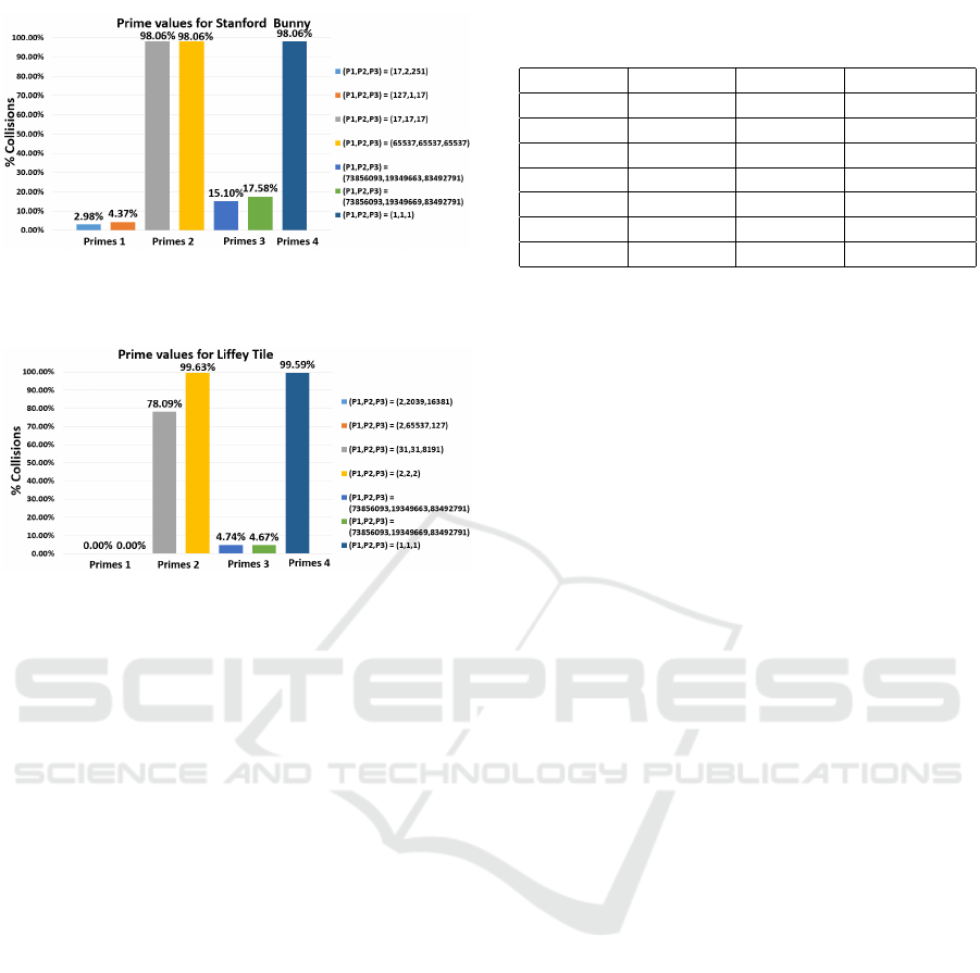
Figure 2: Comparison of Prime Values for the Stanford
Bunny.
Figure 3: Comparison of Prime Values for the Liffey Tile.
less than 83492791, the largest of the primes sug-
gested by (Teschner et al., 2003) were considered.
2040 and 128000 Hash Table Entries were used re-
spectively. These table sizes were chosen as they
equate to roughly half the total number of voxels in
each of these datasets.
A subset of the results obtained from testing vari-
ous primes for the Stanford Bunny and the Liffey Tile
are shown in Figures 2 and 3 respectively. These re-
sults were chosen to demonstrate how the choice of
primes can greatly influence the addressing collision
rate. The following combinations are displayed:
1. Prime combinations that produced the lowest ad-
dressing collision rates (Primes 1)
2. Prime combinations that produced the highest ad-
dressing collision rates (Primes 2)
3. Prime combinations used in (Teschner et al.,
2003; Eitz and Lixu, 2007; Niener et al., 2013)
and (K
¨
ahler et al., 2015) (Primes 3)
4. All prime values set to one (Primes 4)
It was found that the primes used in (Teschner
et al., 2003) and (Eitz and Lixu, 2007), and those
used in (Niener et al., 2013) and (K
¨
ahler et al.,
2015) achieved an addressing collision rate which was
higher than other combinations of primes. It was
found, as is evident from Figures 2 and 3, that many
combinations of primes provided the minimum num-
ber of addressing collisions, i.e. 0% for the Liffey
Table 2: Testing of various combinations of ordering of
primes on the Stanford Bunny.
Bunny
P
1
P
2
P
3
% Collisions
73856093 19349663 83492791 15.09
73856093 83492791 19349663 17.39
83492791 73856093 19349663 16.81
83492791 19349663 73856093 16.78
19349663 83492791 73856093 16.32
19349663 73856093 83492791 17.51
tile, and very low rates (2.98%) for the Bunny. While
these values are still primes, they are not all “large
primes” as stipulated in (Klingensmith et al., 2015).
These results indicate that “large primes” are not
required to achieve optimal results for XOR hashing
for volumetric data.
5.2 Comparison of the Ordering of
Prime Values for XOR Hashing
Another observation is that none of (Teschner et al.,
2003; Niener et al., 2013; Eitz and Lixu, 2007)
or (K
¨
ahler et al., 2015) discuss the ordering of the
prime utilised, i.e. which of the primes are assigned
to (P
1
, P
2
, P
3
) respectively.
To investigate whether varying the order of the
primes would impact the addressing collision rate,
the order of the primes from (Teschner et al., 2003)
and (Eitz and Lixu, 2007) were varied for the Stanford
Bunny. These results are shown below in Table 2.
While the collision rates did not vary greatly for
the primes used in Table 2, other prime values pro-
duced greater variance. Testing ordering combina-
tions of (P
1
, P
2
, P
3
) = (2, 17, 127) for the Stanford
Bunny produced addressing collision rates of between
6.02% and 16.10%.
These results indicate that not only does the choice
of primes impact the addressing collision rate for
XOR Hashing, so too does the ordering of those
primes.
5.3 Comparison of Non Prime Values
for XOR Hashing
Upon the discovery in Section 5.2 that large primes
are not necessary to optimally hash 3D volumetric
data, it was investigated whether there is a need for
the “prime” values used in XOR Hashing to be primes
at all.
The same methodology as described in Section 5.2
was followed for this test - various non prime values
were used for (P
1
, P
2
, P
3
) from equation 3 for XOR
GISTAM 2018 - 4th International Conference on Geographical Information Systems Theory, Applications and Management
308
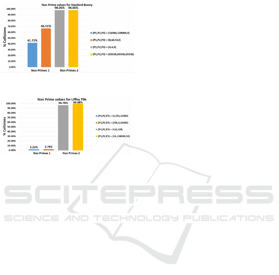
Figure 4: Comparing non prime values on the Stanford
Bunny.
Figure 5: Comparing non prime values on the Dublin City
Dataset Liffey Tile.
Hashing. These were again tested on the Stanford
Bunny (Turk and Levoy, 2005) and the Liffey Tile
from the Dublin City Dataset (Laefer et al., 2015). To
ensure that the values tested were not primes, powers
of 2 were used, up to 2
17
. A subset of these results
are shown in Figures 4 and 5. These results were cho-
sen to demonstrate how the choice of non primes can
greatly influence the addressing collision rate. The
following combinations are displayed:
1. Non Prime combinations that produced the lowest
addressing collision rates (Non Primes 1)
2. Prime combinations that produced the highest ad-
dressing collision rates (Non Primes 2)
Testing with non prime values for XOR Hashing
provided mixed results. While addressing collision
rates of < 3% were obtained using non prime values
for the Liffey Tile, the lowest rate obtained for the
Stanford Bunny was 41.72%.
While using non prime values for the Liffey Tile
did not produce addressing collision rates as low as
when using some prime combinations, it produced
better results than using (P
1
, P
2
, P
3
) from (Teschner
et al., 2003; Eitz and Lixu, 2007), and (Niener et al.,
2013; K
¨
ahler et al., 2015). However, non prime val-
ues for the Stanford Bunny did not produce address-
ing collision rates lower than when using (P
1
, P
2
, P
3
)
from (Teschner et al., 2003; Eitz and Lixu, 2007),
and (Niener et al., 2013; K
¨
ahler et al., 2015).
This indicates that while non prime values for
XOR Hashing can provide better results than using
primes for some datasets, one cannot definitely say
that using primes/non primes is favorable over using
the other.
5.4 Determination of the Influence of
the Choice of Constant Values on
the Distribution of Addressing
Collisions
The distribution of collisions could be of concern de-
pending on the application. For example, a large con-
centration of collisions in one place could lead to the
loss of say an entire object in an indoor environment
when using hashing for SLAM applications. This
could be problematic for an indoor robot scanning a
living room if collisions occurred for all the voxels
associated with a chair. However, if the collisions are
better distributed, only a number of addressing col-
lisions may occur from a few objects. It is therefore
important to determine if certain combinations of con-
stant values can provide well distributed addressing
collisions for a range of 3D volumetric data.
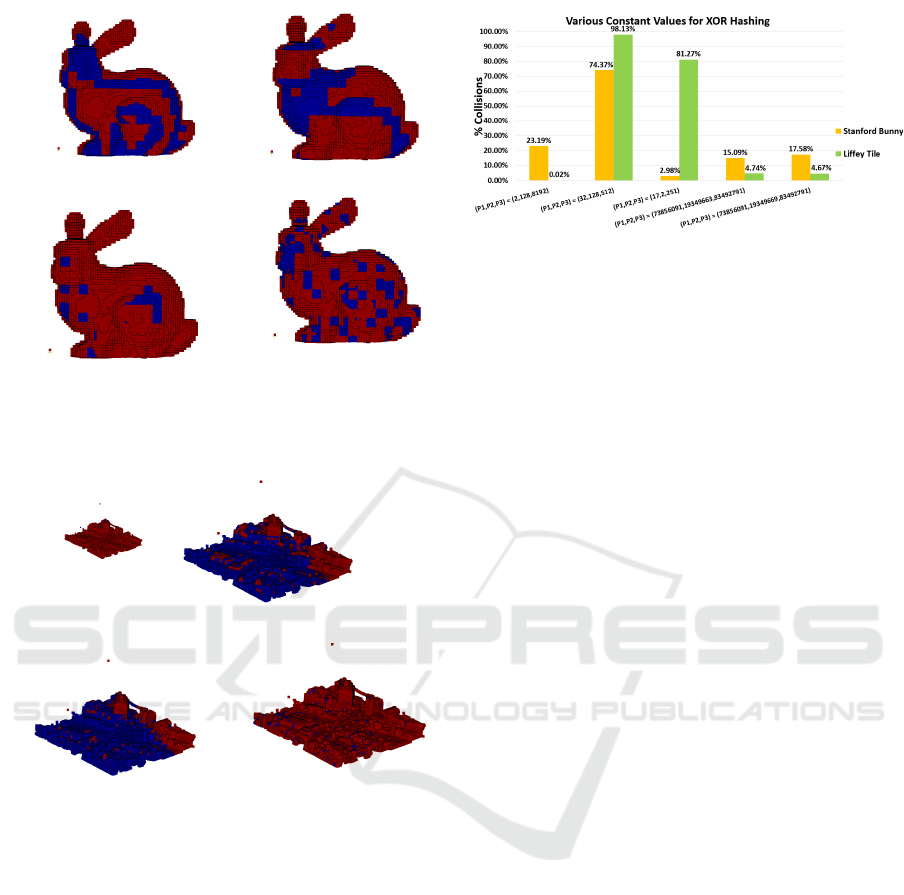
A visual representation for the collision rates us-
ing the constant values from Section 5.5 are shown
in Figures 6 and 7 for both the Stanford Bunny (Turk
and Levoy, 2005) and the Liffey Tile from the Dublin
City Dataset (Laefer et al., 2015). These figures indi-
cate the distribution of addressing collisions for both
models, and how these distributions can be influenced
by the constant values chosen for XOR Hashing. In
Figures 6 and 7 red voxels represent voxels that are
inserted into the hash table successfully. Blue voxels
represent where an addressing collision occurred and
thus the voxels could not be inserted.
What is apparent from these results is not only
does the choice of constants for (P
1
, P
2
, P
3
) signifi-
cantly impact the addressing collision rate of XOR
Hashing, it also impacts the distribution of collisions.
This is more apparent from Figure 6 than Figure 7
as the resolution is smaller (64
3
voxels v 256
3
). In
Figures 6a and 6b, the majority of collisions that oc-
cur are grouped together. However, in Figures 6c,
and 6d, while the percentage of addressing collisions
are lower, the collisions that do occur are for the most
part well distributed across the model.
However, one cannot draw definitive conclusions
from the distribution of collisions in Figure 6, as the
same is not necessarily true in Figure 7. Figure 7c
uses the same constants as in Figure 6c, but with a far
higher addressing collision rate (81.27% v 2.98%),
and thus cannot provide well distributed collisions for
Investigating the Use of Primes in Hashing for Volumetric Data
309
(a) (P
1
, P
2
, P
3
) = (2, 128, 8292)
(b) (P
1
, P
2
, P
3
) = (32, 128, 512)
(c) (P
1
, P
2
, P
3
) = (17, 2, 251)
(d) (P
1
, P
2
, P
3
) =
(73856093, 19349663, 83492791)
Figure 6: Comparing different combinations of constant
values for XOR Hashing on the Stanford Bunny (Turk and
Levoy, 2005).
(a) (P
1
, P
2
, P
3
) =
(2, 128, 8292)
(b) (P
1
, P
2
, P
3
) = (32, 128, 512)
(c) (P
1
, P
2
, P
3
) = (17, 2, 251)
(d) (P
1
, P
2
, P
3
) =
(73856093, 19349663, 83492791)
Figure 7: Comparing different combinations of constant
values for XOR Hashing on the Liffey Tile from the Dublin
City Dataset (Laefer et al., 2015).
the Liffey Tile in Figure 7c as the collision rate is so
high.
While the constants used in Figures 6d and 7d do
provide well distributed addressing collisions, there
are constant value combinations that provide a lower
addressing collision rate for the two models.
It is thus determined that while certain constant
value combinations provide well distributed address-
ing collisions for the two models tested, these val-
ues do not necessarily provide the lowest possible ad-
dressing collision rate.
Figure 8: Comparing different constant values for XOR
Hashing for the Stanford Bunny and the Liffey Tile from
the Dublin City Dataset.
5.5 Determination of Whether
“Optimum Values” Exist for XOR
Hashing
In Section 5.2 it was shown that large primes are
not necessary to minimise addressing collisions for
XOR hashing - smaller primes produced less address-
ing collisions than the large primes recommended
in (Teschner et al., 2003) and (Eitz and Lixu, 2007).
In Section 5.3 it was shown that for the Liffey Tile,
small, non prime values can produce far fewer ad-
dressing collisions for XOR hashing when compared
with the large primes recommended in (Teschner
et al., 2003), (Eitz and Lixu, 2007), (Niener et al.,
2013) and (K
¨
ahler et al., 2015). However, this did
not hold true for the Stanford Bunny.
On the back of both of these findings, it was then
investigated whether one set of constant values for
(P
1
, P
2
, P
3
) in XOR Hashing can provide optimal re-
sults regardless of the 3D volumetric data being con-
sidered. All of (Teschner et al., 2003; Klingensmith
et al., 2015; Niener et al., 2013; Eitz and Lixu, 2007;
K
¨
ahler et al., 2015) use large primes for XOR Hash-
ing for 3D volumetric data, but do not consider, in
detail, how the nature of the data could influence the
choice of constants, be they primes or not.
To determine whether a set of values could be used
in XOR hashing that would provide adequate results
for a diverse range of 3D volumetric data, various
combinations of primes and non primes were tested
for the Stanford Bunny (Turk and Levoy, 2005) and
the Liffey Tile of the Dublin City Dataset (Laefer
et al., 2015). The results are shown below in Figure 8.
These values were also tested on the whole Dublin
City Dataset (Laefer et al., 2015) and the New York
Dataset (of Commerce, 2014a), the results of which
are shown in Figures 9 and 10 respectively in the form
of a box-plot.
From Figure 8 it is clear that constant values
that provide a low addressing collision rate for one
GISTAM 2018 - 4th International Conference on Geographical Information Systems Theory, Applications and Management
310
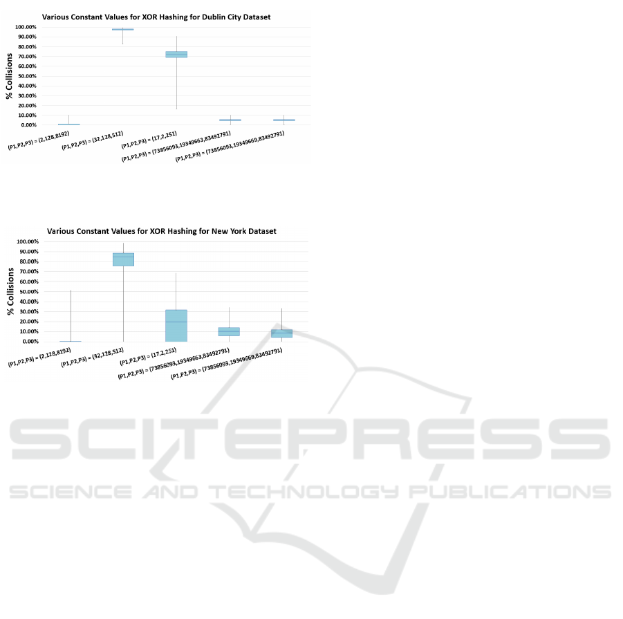
Figure 9: Comparing different constant values for XOR
Hashing for the Dublin City Dataset.
Figure 10: Comparing different constant values for XOR
Hashing for the New York City Dataset.
model do not guarantee a low collision rate for an-
other model. This is of importance as the distribution
of voxels in models being considered is not always
known before hashing.
Figures 9 and 10 indicate again that varying
constant values cannot be guaranteed to provide a
low addressing collision rate for a wide range of
datasets. The results for (P
1
, P
2
, P
3
) = (2, 128, 8192)
and (P
1
, P
2
, P
3
) = (73856093, 19349663, 83492791)
in both Figures 9 and 10 are statistically significant as
there is no overlap between the distributions. These
results also indicate that the constant values recom-
mended in (Teschner et al., 2003; Eitz and Lixu, 2007;
Niener et al., 2013) and (K
¨
ahler et al., 2015) do not al-
ways provide the lowest possible addressing collision
rate.
It was thus determined that there is no set of “op-
timum values” that can be used to optimally hash
a wide range of 3D volumetric datasets using XOR
Hashing, and it is unwise to advise the use of certain
values over others without prior knowledge of the data
to be hashed.
6 CONCLUSION
The following have been determined regarding the
use of primes for the hashing of 3D volumetric data
through the research conducted as part of this paper:
• Primes (large or otherwise) are not required in
XOR Hashing for optimal results - non primes can
provide equal and at times better addressing colli-
sion rates.
• The ordering of primes in XOR Hashing impacts
the addressing collision rate.
• When primes are used in XOR hashing, larger
primes do not necessarily produce optimal results.
More specifically, the primes used in (Teschner
et al., 2003; Klingensmith et al., 2015; Niener
et al., 2013; Eitz and Lixu, 2007) and (K
¨
ahler
et al., 2015) do not necessarily produce optimal
results.
• The choice of constant values in XOR Hashing in-
fluences the distribution of addressing collisions.
However, the constants that provide the highest
distribution of addressing collisions do not neces-
sarily provide the lowest percentage of addressing
collisions.
• No one set of values, primes or otherwise, for
XOR Hashing can be considered to provide op-
timal results due to the variance that exists across
different 3D volumetric datasets.
Given the results above, it is the view of the au-
thors of this paper that XOR hashing is not the op-
timal method to hash 3D volumetric data due to the
variance that exists with 3D volumetric data, more
specifically with dynamic 3D volumetric data. This
is due to the need to predefine values for (P
1
, P
2
, P
3
),
at times without any prior knowledge of the distribu-
tion of the voxels in the data that needs to be hashed.
A dynamic method, that could adapt to the distribu-
tion of voxels within models would provide more pre-
dictability while hashing 3D volumetric data.
REFERENCES
Carter, J. L. and Wegman, M. N. (1979). Universal classes
of hash functions. Journal of computer and system
sciences, 18(2):143–154.
Dumey, A. I. (1956). Indexing for rapid random ac-
cess memory systems. Computers and Automation,
5(12):6–9.
Eitz, M. and Lixu, G. (2007). Hierarchical spatial hashing
for real-time collision detection. In Shape Modeling
and Applications, 2007. SMI’07. IEEE International
Conference on, pages 61–70. IEEE.
Investigating the Use of Primes in Hashing for Volumetric Data
311

Good, I. J. (1950). Probability and the weighing of evi-
dence.
Jaeschke, G. (1981). Reciprocal hashing: A method for
generating minimal perfect hashing functions. Com-
munications of the ACM, 24(12):829–833.
K
¨
ahler, O., Prisacariu, V., Valentin, J., and Murray, D.
(2016). Hierarchical voxel block hashing for efficient
integration of depth images. IEEE Robotics and Au-
tomation Letters, 1(1):192–197.
K
¨
ahler, O., Prisacariu, V. A., Ren, C. Y., Sun, X., Torr, P.,
and Murray, D. (2015). Very high frame rate vol-
umetric integration of depth images on mobile de-
vices. IEEE transactions on visualization and com-
puter graphics, 21(11):1241–1250.
Klingensmith, M., Dryanovski, I., Srinivasa, S., and Xiao,
J. (2015). Chisel: Real time large scale 3d reconstruc-
tion onboard a mobile device using spatially hashed
signed distance fields. Robotics: Science and Systems
XI.
Knott, G. D. (1975). Hashing functions. The Computer
Journal, 18(3):265–278.
Knuth, D. E. (1998). The art of computer programming:
sorting and searching, volume 3. Pearson Education.
Laefer, D. F., Abuwarda, S., Vo, A.-V., Truong-Hong, L.,
and Gharib, H. (2015). 2015 aerial laser and pho-
togrammetry survey of dublin city collection record.
Laefer, D. F., Abuwarda, S., Vo, A.-V., Truong-Hong, L.,
and Gharibi, H. (2017). Dublin als2015 lidar license
(cc-by 4.0). https://geo.nyu.edu/catalog.
Mirtich, B. (1997). Efficient algorithms for two-phase colli-
sion detection. Practical motion planning in robotics:
current approaches and future directions, pages 203–
223.
Niener, M., Zollhfer, M., Izadi, S., and Stamminger, M.
(2013). Real-time 3d reconstruction at scale us-
ing voxel hashing. ACM Transactions on Graphics,
32(6):111.
of Commerce, U. D. (2014a). 2013-2014 u.s. geo-
logical survey cmgp lidar: Post sandy (new york
city). https://data.noaa.gov/dataset/dataset/2014-u-s-
geological-survey-cmgp-lidar-post-sandy-new-jersey.
Accessed: 2017-10-05.
of Commerce, U. D. (2014b). Post sandy lidar survey li-
cense. https://data.noaa.gov/dataset/dataset/2014-u-s-
geological-survey-cmgp-lidar-post-sandy-new-jersey.
Accessed: 2017-10-19.
Sprugnoli, R. (1977). Perfect hashing functions: a single
probe retrieving method for static sets. Communica-
tions of the ACM, 20(11):841–850.
Teschner, M., Heidelberger, B., Mller, M., Pomeranets, D.,
and Gross, M. (2003). Optimized spatial hashing for
collision detection of deformable objects. 3.
Turk, G. and Levoy, M. (2005). The stanford bunny.
APPENDIX
A DATASETS
The following datasets were examined in the com-
parison of various hashing techniques as described
in Section 4. The datasets include small scale syn-
thetic models and publicly available large scale Li-
DAR datasets. The large scale models present a real-
istic representation of what would be processed by an
embedded system in the real world, except on a much
larger scale.
• Stanford Bunny. The Stanford Bunny is a widely
used 3D test model developed by Greg Turk and
Marc Levoy in 1994 at Stanford University (Turk
and Levoy, 2005).
• Dublin City Dataset. The Dublin City Dataset is
a collection of LiDAR scans of Dublin City (Lae-
fer et al., 2015; Laefer et al., 2017).The scans are
separated into tiles. Each of these tiles are 256
3
voxels, 100m on a side. The average occupancy
of the Dublin City Dataset is 1.36%.
• Liffey Tile from The Dublin City Dataset. This
tile was used in some tests. It was chosen as it
is representative of the other tiles in the dataset,
and is named the Liffey Tile as it shows the Liffey
river flowing under the iconic O’Connell Bridge
in Dublin’s city centre.
• New York Dataset. The New York Dataset refers
to the 2014 U.S. Geological Survey CMGP Li-
DAR: Post Sandy (New Jersey) (of Commerce,
2014a; of Commerce, 2014b). This dataset is also
a collection of Lidar scans of New York and New
Jersey. Each of these tiles are 64
3
voxels, 100m
on a side, equating to 10, 000m
3
. The average oc-
cupancy of the New York Dataset is 2.64%.
GISTAM 2018 - 4th International Conference on Geographical Information Systems Theory, Applications and Management
312
