Evaluating the Complementarity of Communication Tools

for Learning Platforms

Leonardo Carvalho

, Laura Assis

, Leonardo Lima

, Eduardo Bezerra

, Gustavo Guedes

Artur Ziviani

, Fabio Porto

, Rafael Barbastefano

and Eduardo Ogasawara

Federal Center for Technological Education of Rio de Janeiro, CEFET/RJ, Brazil

National Laboratory for Scientiﬁc Computing, LNCC, Brazil

Keywords:

Social Media, Evaluation, Learning Platforms, Communication Tools.

Abstract:

Due to the constant innovations in communications tools, several educational institutions are continually eva-

luating the adoption of new communication tools (NCT) for their adopted learning platforms (LP). Notably,

many educational institutions are interested in checking if NCT is bringing beneﬁts in their teaching and le-

arning process. We can state an important problem that tackles this interest as for how to identify when NCT

is providing a signiﬁcantly different complementary communication ﬂow concerning the current communi-

cation tools (CCT) provided at LP. This paper presents the Mixed Graph Framework (MGF) to address the

problem of measuring the complementarity of an NCT in the scenario where some CCT is already established.

Since we are interested in the methodological process, we evaluated MGF using synthetic data. Our experi-

ments observed that the MGF was able to identify whether an NCT produces signiﬁcant changes in the overall

communications of an LP according to some centrality measures.

1 INTRODUCTION

Communication tools are in constant evolution. They

usually change the way people collaborate with each

other. Not long ago, letters, telegrams, and other writ-

ten communications on paper were the mainstream.

However, since the beginning of the Internet, com-

munication tools were extended through e-mail. The

use of e-mail is widespread and almost ubiquitous in

educational institutions, being responsible for the ma-

jority of the communication ﬂow inside them (Kola-

czyk, 2009).

Innovations in communication tools continue to

occur, and several new features, such as instant mes-

saging, blogs, and content management have been

developed. Recently, new opportunities to empower

communication among students-teachers have arisen

with the advent of online learning platforms (LP)

(Moore et al., 2011). There is some specialized LP,

such as Moodle that can be customized and extended

(Kellogg et al., 2014). Inside LP, instant messaging

(IM), wikis, and other social applications can be bet-

ter options for collaborative work and are, thus, gai-

ning momentum in scholarly communications tasks

(Mazzolini and Maddison, 2003).

As an emerging communication technology, on-

line social networks provide a variety of communica-

tion services such as proﬁles, comments, private mes-

saging, blogging, media ﬁle sharing, and instant mes-

saging. Some of these communication tools provide

their services through a mobile network (Chai and

Kim, 2012). These features are important as they help

to break existing barriers to communication among

members. They can stimulate interactions involving

student-teacher.

Due to demands of privacy and other pedagogical

decisions, educational institutions also may choose to

establish private social networks that are integrated

to LP and restricted to student-teacher of their main

courses. These tools are commonly inspired on pu-

blic social networks, such as Facebook, LinkedIn, in-

cluding Web 2.0/3.0 collaboration tools. In particu-

lar, they have to focus on educational issues, such

as improvement course interactions between teacher-

student and better integration with other educational

tools.

The choice for a particular LP and their customi-

zations can be both time-consuming and expensive.

Under this perspective and due to investments, edu-

cational institutions are concerned to measure the ef-

fective adoption of a new communication tool (NCT).

They are thus searching for an efﬁcient way to as-

sess if an NCT is bringing beneﬁts for their LP. We

can state the problem as of how to identify when an

NCT is providing a communication ﬂow that is com-

plementary to the current communication tool (CCT)

142

Carvalho, L., Assis, L., Lima, L., Bezerra, E., Guedes, G., Ziviani, A., Porto, F., Barbastefano, R. and Ogasawara, E.

Evaluating the Complementarity of Communication Tools for Learning Platforms.

DOI: 10.5220/0006798701420153

In Proceedings of the 10th International Conference on Computer Supported Education (CSEDU 2018), pages 142-153

ISBN: 978-989-758-291-2

being used in LP.

In this paper, we address the problem of measu-

ring the complementarity of a NCT in the scenario

where some CCT is already an established in LP. In

order to do that, we present the Mixed Graph Frame-

work (MGF), which is a network obtained by a mix

of the CCT and the NCT networks, and is designed

to evaluate how a new complementar communication

tool can change the process of exchanging informa-

tion throughout the network. The proposed MGF is

based on the premise that the CCT can be conside-

red as a baseline for evaluating any other tool to im-

prove communication in educational institutions LP.

It is important to use a common standard represen-

tation of the communication ﬂow to enable compa-

rison between them. In this work, the communica-

tion networks from the CCT and the NCT are mo-

deled as graphs, named G

and G

, respectively. From

these graphs, the MGF produces a mixed graph G

measure if a NCT is acting as a complementary tool

among students as compared with the CCT.

We have evaluated MGF using synthetic data that

represents teacher-students communication ﬂows. In

our experiment, we assume the usage of a Moodle-

like LP that is mainly adopting course messages as

CCT and Social Network plugin as NCT. Based on

the shared messages in both tools, we compute several

metrics and conduct a statistical analysis on them to

evaluate the complementarity of the NCT. Our expe-

riments observed that the MGF was able to identify

whether an NCT produces signiﬁcant changes in the

overall communication.

The remainder of the paper is organized as fol-

lows. Sections 2 and 3 present related work and the

general background, respectively. The proposed MGF

is described in Section 4. Section 5 presents our expe-

rimental evaluation. Finally, Section 6 concludes the

paper.

2 RELATED WORK

The analysis of social networks is widely explored,

and it has been studied for several years (Ngai et al.,

2015). Many of these studies focused on the informa-

tion that can be extracted from these networks ana-

lyzing their dynamics and structure. When it co-

mes to the impacts of communication tools adoption

in an educational environment, the need for study

in this area expanded in recent years (Chatti et al.,

2007; Hrastinski, 2009; Cadima et al., 2010; Kellogg

et al., 2014). These studies focus on the effects of the

usage of social network tools in LP and the learning-

teaching achievements (Siribaddana, 2014).

One of the main concerns about the adoption of

communication tools is related to the notion of being

social (Wasko et al., 2009). We can ﬁnd several pu-

blications on the use of open social networks, most

of them representing the information ﬂow as a graph.

In such background, it is possible to extract metrics

that enables data mining (Nettleton, 2013), such as

groups identiﬁcation (clusters or cliques) that are re-

lated to concentrations of communication ﬂows inside

the graph (Prado and Baranauskas, 2013). Many of

these metrics, such as cohesion and average distance,

are useful in network analysis, as they enable insights

about the communication ﬂows (Newman, 2003).

In some studies, the authors structure and compare

social networks by analyzing the communication ﬂow

among students of courses available in a Distance Le-

arning Scenario (Hamulic and Bijedic, 2009; Siribad-

dana, 2014). Their research showed that the data from

these social tools could be used to analyze the com-

munication ﬂow and draw conclusions to improve the

available e-learning courses.

Some researchers have proposed frameworks for

understanding social media (Kellogg et al., 2014;

Chai and Kim, 2012) that suggest a theoretical frame-

work to understand social networking site users’ kno-

wledge contribution behavior and inter-relationships

among different research constructs adopted (Ngai

et al., 2015).

Many works analyze social networks and study its

behavior. Also, some papers propose frameworks for

these purposes. Nonetheless, as far as we know no ot-

her work suggests a Mixed Graph framework to mea-

sure if an NCT is complementary to a CCT already in

use in an LP.

3 BACKGROUND

This section presents the fundamental concepts for

the paper and is organized into three main subsecti-

ons. Section presents general graph concepts. Section

describes the major centrality-based measures that are

used as input for the performed statistical analysis.

Section presents the general statistical tests for non-

parametric data sets.

This section presents the fundamental concepts for

the paper and is organized into three main subsecti-

ons. Section 3.1 presents general graph concepts.

Section 3.2 describes the major centrality-based mea-

sures that are used as input for the performed statisti-

cal analysis. Section 3.3 presents the general statisti-

cal tests for non-parametric data sets.

Evaluating the Complementarity of Communication Tools for Learning Platforms

143

3.1 Graph Representation

Using graph theory terminology (Ahuja et al., 1993),

communication networks (such as LP and LP) can be

modeled as a weighted directed graph G(V, E), where

V is the set of |V| nodes and E is the set of |E| edges.

A node i ∈V represents a member with a connection

point. The arcs (i, j) ∈ E, i ∈V and j ∈V represent a

communication link between two members.

A weight w

i j

> 0 is assigned to each edge with

ending nodes i and j and represents the amount of

communication ﬂow between these two nodes. Since

G(V,E) is directed, it may be that w

i j

6= w

. The ad-

jacency matrix A

i, j

= a

i, j

of the weighted graph G can

be deﬁned as:

i j



i j

, if an edge is connecting node i to j

0, otherwise.

3.2 Graph Centrality Measures

When some problem is modeled by a graph, many

properties are associated with each node, such as dis-

tance and centrality. These properties provide a sum-

mary of the graph.

A general centrality measure is the weighted clo-

seness of a node v (Opsahl et al., 2010). If a node v re-

presents a member in an educational network, the clo-

seness of v measures how close a member is to others.

Collaborators that occupy central positions concer-

ning closeness are important in communication (Was-

serman and Faust, 1994). The weighted closeness of a

node v is computed by C

(v) =

∑

x ∈ V \v

d(v,x)

, where

d(v,x) is the weighted geodesic distance between the

nodes v and x.

Another well-known measure is the weighted bet-

weenness centrality of a node v (Kolaczyk, 2009). It is

a measure aimed at summarizing the extent to which

a vertex is located ‘between’ other pairs of vertices.

Let us introduce some notation before formally deﬁne

the betweenness centrality. Consider arbitrary nodes

u,v ∈V. A path P(u, v) which starts at u and ﬁnishes

at v is an ordered sequence of nodes, P(u, v) = <

u = v

,.. .,v

= v >, such that e

= (v

i+1

) ∈E

for i = 1,..., k−1. The length of the path P(u,v) is gi-

ven as the sum of the edge weights of the path and the

shortest path function s

(u,v) between nodes u,v ∈V

is given by s

(u,v) = min

P(u,v)

∑

k−1

i=1

i,i+1

. The be-

tweenness centrality for any given node v ∈V is then

given by C

(v) =

∑

s6=t6=v∈V

σ(s,t|v)

σ(s,t)

, where σ(s,t) is the

number of paths P(s,t) of size s

(s,t) connecting s

and t and σ(s,t|v) is the number of shortest paths pas-

sing through vertex v.

The third class of centrality measure is the Klein-

berg centrality (Kleinberg, 1999). The main idea is

to identify nodes that correspond to hubs and autho-

rities. A hub is a node that points to many relevant

nodes, and an authority node is the one that is poin-

ted by many important nodes. Both are based on the

eigenvectors related to the largest eigenvalues of the

matrices AA

and A

A. The hub centrality of the node

, denoted here byC

), is the i−th entry of the vec-

tor x satisfying AA

x = λx, where λ ∈ ℜ is the largest

eigenvalue of AA

Similarly, the authority of a node v

, denoted here

by C

), is the i−th entry of the vector y satisfying

Ay = βy, where β ∈ ℜ is the highest eigenvalue of

3.3 Statistical Analysis

The need to compare two different datasets is wide-

spread. Such comparison may vary according to the

objectives of the study. We can summarize two diffe-

rent statistical tests that are relevant to compare two

data sets: (i) distribution; and (ii) correlation (Larsen

and Marx, 2005). For each one of these scenarios,

there is a set of statistical tests that can be used. They

vary according to the distribution of the data sets.

Commonly, social medias are scale-free networks and

follow a power-law distribution. In this case, non-

parametric tests are more adequate. For the sake of

simplicity, we are going to present one statistical test

for comparing two data sets.

Mann-Whitney U test, also known as Wilcoxon

rank sum test from the difference in medians, is a

distribution analysis test. The goal of this test is to

measure the extent to which the medians of two inde-

pendent data sets are different from each other, i.e., to

check if the difference between the median of these

two data sets is signiﬁcantly different from zero.

Spearman rank correlation test is a correlation

analysis test, whose goal is to test if the rank correla-

tion coefﬁcient between two variables is signiﬁcantly

different from zero. The null hypothesis establishes

zero correlation between two variables.

4 MGF

In this section, we present a framework to evaluate

the complementarity of communication tools using a

mixed graph modeling, called here Mixed Graph Fra-

mework (MGF). Algorithm 1 summarizes how the

MGF works. The ﬁrst two lines (2-3) are related

to modeling graphs for communication tools and are

described in further detail in Section 4.1. Line (4)

is described in Section 4.2 and produces the mixed

CSEDU 2018 - 10th International Conference on Computer Supported Education

144

graph. Line (5) is described in Section 4.3 and com-

putes centrality measures to evaluate the complemen-

tarity of the NCT concerning the CCT.

4.1 Extract Functions

The ﬁrst two activities of Algorithm 1 encompass mo-

deling graphs from the communication tools. Graphs

= (V

) and G

= (V

) are, respectively,

generated through the extraction Functions f Extract

and f Extract

that are applied over the CCT and NCT

datasets.

A node i ∈ V

and p ∈ V

corresponds to mem-

bers of their respective graphs G

and G

. An edge

i, j

∈ E

represents a communication in CCT from

member i ∈V

to member j ∈V

and the edge weight

(i, j) corresponds to the number of messages ex-

changed from i to j. Similarly, an edge e

i, j

∈ E

re-

presents a communication in the NCT from member i

to member j ∈V

and the edge weight w

(i, j) corre-

sponds to the number of messages exchanged from i

to j.

Both f Extract

and f Extract

are User Deﬁned

Functions (UDFs) that vary according to the adop-

ted communication tools. For example, if CCT corre-

sponds to course messages in an LP tool, the commu-

nication ﬂow in the graph G

between two members i

and j ∈V are measured by the number of posts messa-

ges exchanged by them, as described in Equation (1).

On the other hand, if the NCT is an LP tool, the com-

munication ﬂow is measured by the weighted average

of comments and likes someone is interested in ex-

tracting from the LP, as described in Equation (2).

Algorithm 1: Main MGF Algorithm.

1: function MGF(D d

, D d

, e f

)

2: G

← fExtract

)

3: G

← fExtract

)

4: G

← fMix(G

, G

)

5: return fAnalyze(G

, G

)

6: end function

1: function fAnalyze(G

, G

)

2: r

← analyzeClosenessDist(G

, G

)

3: r

← analyzeClosenessCorr(G

, G

)

4: r

← analyzeBetweennessCorr(G

, G

)

5: r

← analyzeEigenTopK(G

, G

)

6: return {r

}

7: end function

(i, j) = |posts(i, j)| (1)

(i, j) =

β|comments(i, j)| + γ|likes(i, j)|

β + γ

(2)

Figures 1(a) and 1(b) display illustrative examples

of G

and G

, respectively. The graph G

is obtai-

ned by applying f Extract

over the D

dataset and

the graph G

is obtained by applying f Extract

over

dataset.

A E

(a)

A E

1 3

(b)

A E

(c)

mixgraphs

Figure 1: Communication ﬂow: (a) G

extracted from the

CCT dataset; (b) G

extracted from NCT dataset; (c) G

produced by mixing G

with G

4.2 Mixed Graphs

Let G

= (V

) be the mixed graph with node set

= V

of order |V

| and edge set E

∪E

. To each edge e

i, j

∈ E

a weight w

(i, j) is

assigned as given by Equation (3). The mixed graph

activity is described in Algorithm 2. It receives both

and G

as an input and builds the mixed graph

of order |V

| with its edges weights given by the

vector w

(i, j) = w

(i, j) + w

(i, j) (3)

Note that the graph G

represents the total ﬂow of

communication provided by the two communication

tools and can be used to identify whether the NCT

is changing the communication ﬂow or just mirro-

ring the communication ﬂows between members in

the CCT. An example of G

can be observed in Fi-

gure 1(c) obtained from G

and G

Evaluating the Complementarity of Communication Tools for Learning Platforms

145

Algorithm 2: Mixed Graphs.

1: function fMix(G

, nG)

2: V

←V

∪V

3: G

← EmptyGraph(|V

4: for i ← 1 to |V

| do

5: for j ← 1 to |V

| do

6: if i <> j then

7: w

(i, j) ← w

(i, j) + w

(i, j)

8: end if

9: end for

10: end for

11: return (mG,w

)

12: end function

4.3 Complementarity Analysis

The complementarity analysis computes centrality

measures of each vertex extracted from G

and G

These values are used to compute if such metrics from

are statistically signiﬁcantly different from G

. In

this case, it indicates that G

is not simply an overlap

of G

, i.e., actually bringing complementarity in the

overall communication. Such an activity is described

in Algorithm 3.

Algorithm 3: Analysis of Centrality.

1: function analyzeClosenessDist(G

, G

)

2: vc

← closeness(convertDist(G

))

3: vc

← closeness(convertDist(G

))

4: return wilcox.test(vc

,vc

)

5: end function

1: function analyzeClosenessCorr(G

, G

)

2: vc

← closeness(convertDist(G

))

3: vc

← closeness(convertDist(G

))

4: return spearman.cor.test(vc

,vc

)

5: end function

1: function analyzeBetweennessCorr(G

, G

)

2: vb

← betweenness(convertDist(G

))

3: vb

← betweenness(convertDist(G

))

4: return spearman.cor.test(vb

,vb

)

5: end function

1: function analyzeHub(G

, G

,k)

2: ve

← eigen(asHub(convertDist(G

)))

3: ve

← eigen(asHub(convertDist(G

)))

4: ratio ←overlap(top

(ve

),top

(ve

))

5: sig ← hgeo(ratio,k ·|ve

|,(1−k) ·|ve

6: return {ratio, sig}

7: end function

It is worth mentioning that all centrality-based

measures expect a weighted adjacency matrix as an

input. However, in all built graphs (G

, G

, and G

the weight of the edges corresponds to the commu-

nication ﬂow over a period. In this way, prior to

any centrality computation, it is important to con-

vert ﬂows to distances since more messages, e-mails,

and post exchanges imply less distance between two

members. Such a transformation is described by

Function convertDist(w) that applies Equation (4) for

all edges in Algorithm 3.

w(i, j) =

w(i, j)

(4)

Functions closeness, betweenness, and Eigen, re-

spectively compute the weighted closeness, weigh-

ted betweenness, and weighted Eigen vectors measu-

res (Opsahl et al., 2010) of G

and G

. The ﬁrst line

in all functions described in Algorithm 3 is to convert

the communication-based graph into a distance-based

graph according to Equation (4).

Function analyzeClosenessDist analyzes the clo-

seness centrality distribution. The goal is to compute

if the difference in the median of the closeness of each

graph is signiﬁcantly different from zero. For that,

the nonparametric Wilcoxon rank sum is used (De-

vore and Berk, 2011). The intuition of this function

is to compute if the introduction of NCT changes the

amount of communication ﬂow signiﬁcantly concer-

ning the CCT.

Functions analyzeBetweennessCorr and

analyzeClosenessCorr correlate the betweenness

and the closeness centralities between G

and G

respectively. For that, the nonparametric Spearman

correlation test is used (Devore and Berk, 2011).

The intuition of these functions is to compute if

the introduction of the NCT changes signiﬁcantly

the way people interact concerning the CCT by

analyzing the established communication ﬂows.

This indicates if the NCT is not merely increasing

the scale of messages among persons, but if it is

changing the communication ﬂow structure. Such

a test is complementary to analyzeClosenessDist.

We can have situations where analyzeClosenessDist

may not differ but either analyzeClosenessCorr or

analyzeBetweennessCorr may present signiﬁcant

changes and vice-versa.

Function analyzeHub is also a complementary

analysis. It analyzes the inﬂuence of introducing new

edges in the communication ﬂow. It starts by multi-

plying the adjacency matrix with its transpose targe-

ting the main hubs in the communication ﬂow. This is

done in both graphs (G

and G

). Inside the function,

we calculate the top-k more central vertices in both

graphs and the overlap between them (same central

vertices in both graphs). We also compute the pro-

bability using the hypergeometric distribution of such

CSEDU 2018 - 10th International Conference on Computer Supported Education

146

an occurrence.

The MGF is implemented in R. Statistical tests,

such as Wilcoxon rank sum and Spearman correlation

tests, are available in many statistical packages, such

as R (Dalgaard, 2008) and were included in MGF.

5 EXPERIMENTAL EVALUATION

This section presents the evaluation of the proposed

MGF in measuring if the NCT brings complemen-

tarity to the CCT inside a Learning Platform (LP).

We used synthetic data to simulate both CCT and

NCT usage to explore the MGF under different group

conﬁgurations and educational scales. Both MGF

and experimental evaluation is made available at

https://github.com/eogasawara/mgf.

We have organized this section into three parts,

as follows. Section 5.1 discusses synthetic data pre-

paration that models LP (Newman et al., 2002). In

Section 5.2, we describe the general procedure of gro-

wth network used in the experimental evaluation. In

Section 5.3, we present a toy sample analysis to illus-

trate the beneﬁts of MGF. In Section 5.4, we conduct

a sensitive analysis of MGF under different LP scena-

rios.

5.1 Synthetic Data Generation

Many networks can be framed in the deﬁnition of

scale-free networks (Barab

asi and Albert, 1999). A

network is classiﬁed as scale-free if the degree dis-

tribution of its nodes follows the power law mo-

del (Newman et al., 2002). Scale-free networks have

two general concepts: growth and preferential atta-

chment. The idea of growth points out to the con-

stant increase of the number of nodes in the network.

The preferential attachment means that the more con-

nected is a node, the more likely is that it gets new

links. The basic understanding for this second con-

cept is that a new member on the network has a hig-

her probability to interact with a person who interacts

with many people than with someone who is not so

active in the network.

The most notable feature of a scale-free network is

the existence of nodes with degree much higher than

the average degree in the network. The highest degree

nodes are often called hubs and have speciﬁc mea-

nings in each network. The presence of hubs is di-

rectly related to the robustness of the network. Most

of the nodes are not hubs, and the probability of a sig-

niﬁcant impact on total ﬂow with the departure of one

of these low degree nodes is very low. On the other

hand, the removal of a hub can cause a large impact on

the communication ﬂow or even a network partition.

In the experiments presented in our work, we ge-

nerated G

(simulating hierarchical teacher-students

communication) and G

(simulating a social network

communication among all students) as scale-free net-

works. However, G

follows the organizational struc-

ture formed by the traditional teacher-student relati-

onship, whereas the G

does not impose such a con-

straint. This assumption is reasonable since most LP

are organized hierarchically (either teacher-students

or tutors-students).

Algorithm 4 generates synthetic instances of CCT

and NCT; and was implemented using poweRlaw, an

R package to create scale-free graphs. Initially, the

ﬁrst three parameters k,v,e are related to generation

of the subgraphs that will form CCT graph (i.e., G

It starts by creating k subgraphs in G

. Each subgraph

has v nodes with e edges. After that, the most cen-

tral nodes in each subgraph, according to its closeness

centrality, are connected to each other to establish a

hierarchical communication in G

. In the end of G

build phase, this graph has |V

| = v

= v ·k nodes and

|= e

= (e·k)+ k edges. Then, the NCT graph G

is generated with v

= |V

| nodes and e

= |E

| ed-

ges, such that v

= v

. By construction, G

is strictly

scale-free.

Table 1: Parameters used in the experimental evaluation.

Parameter Description

= v

Number of nodes in both graphs,

and G

k Number of groups in G

Number of edges (communication

ﬂows) in G

Number of edges (communication

ﬂows) in G

In Section 5.4, we explore three scenarios produ-

ced during synthetic data generation that correspond

to representative contexts for LP, such as the num-

ber of vertices. A small course has the number of

members greater than 10 and lower than 50, whereas

in medium course the number of members is grea-

ter than or equal to 50 and lower than 250. Additi-

onally, the number of messages and edges explored

in our study are in agreement with communications

using both online social networks (Benevenuto et al.,

2009). The scenarios adopted for LP are presented in

Table 2.

Evaluating the Complementarity of Communication Tools for Learning Platforms

147

1 FIGURES1

(a) G

= 10,k

= 2,e

= 10)(b) G

25%

= 10,e

= 10)(c) G

25%

= G

+ G

25%

(d) G

50%

= 10,e

= 10)(e) G

75%

= 10,e

= 10)(f) G

100%

= 10,e

= 10)

(g) G

50%

= G

+ G

50%

(h) G

75%

= G

+ G

75%

(i) G

100%

= G

+ G

100%

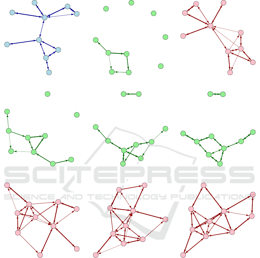
Figure 1.

An example of current tool

(a) and new tool

(b) produced by Algorithm

. The mixed

graph G

is produced by Algorithm ?? from both G

and G

. A network growth for new tool (G

) with

ration equals to 25% (b), 50% (d), 75% (e), and 100% (f); with their respectively effects in producing

mixed graphs (G

), G

25%

(c), G

50%

(g), G

75%

(h), and G

100%

(i). The width of edges are related to their

weights

1/3

Figure 2: An example of current tool G

(a) and new tool G

(b) produced by Algorithm 4. The mixed graph G

is produced

by Algorithm 2 from both G

and G

. A network growth for new tool (G

) with ration equals to 25% (b), 50% (d), 75% (e),

and 100% (f); with their respectively effects in producing mixed graphs (G

), G

25%

(c), G

50%

(g), G

75%

(h), and G

100%

(i).

The width of edges are related to their weights.

5.2 Network Growth

Consider both G

and G

produced during the synt-

hetic dataset production. We can apply the MGF to

compute metrics and check if G

is complementary

to G

. However, to better explore MGF, in all expe-

rimental evaluation we analyzed G

using a network

growth described in Algorithm 5. The goal is to al-

low for the comprehension of the MGF behavior as

we increase G

from an empty graph until reaching

the entire G

structure. According to Algorithm 5,

the growth ratio δ ﬁlter both edge weights and the

number of edges in its entire structure according to

its weight distribution. The edge weights for w

are

CSEDU 2018 - 10th International Conference on Computer Supported Education

148

●

100

0.1

1.0

10 10 10 10 10

degree

frequence

(a)

0% 25% 50% 75% 100%

growth

degree

0% 25% 50% 75% 100%

growth

betweenness

0% 25% 50% 75% 100%

growth

closeness

(b)(c)(d)

●●●●●●●

●

●●●●●

●

●●●●●

●

●●●●●

●

●●●●

●

100

0 10 20 30 40 50 0 10 20 30 40 50 0 10 20 30 40 50 0 10 20 30 40 50 0 10 20 30 40 50

(e)

●

100

0e+00

1e−03

2e−03

2.5e−04 5.0e−04 7.5e−04 1.0e−03 2.5e−04 5.0e−04 7.5e−04 1.0e−03 2.5e−04 5.0e−04 7.5e−04 1.0e−03 2.5e−04 5.0e−04 7.5e−04 1.0e−03 2.5e−04 5.0e−04 7.5e−04 1.0e−03

( f)

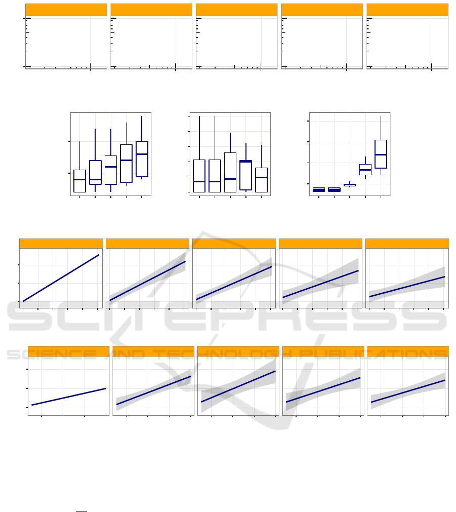
Figure 2. Descriptive statistics of G

in the toy example grouped by growth ratio

d = {0,25,50, 75,100}. The degree distribution of G

is in log x log scale (a). Box-plot of degree (b),

closeness (c), and betweenness (d) distributions of G

. Correlation plot of betweenness (G

x G

) (e).

Correlation plot of closeness (G

x G

) (f)

●● ●● ●● ●● ●● ●● ●● ●● ●●● ●● ●● ●● ●● ●● ●● ●●

●

●● ●

●●

●

●● ●● ●● ●● ●● ●● ●● ●● ●●● ●● ●● ●● ●● ●● ●● ●● ●● ●● ●● ●●

●

●● ●● ●● ●● ●● ●● ●● ●● ●●● ●● ●● ●● ●● ●● ●● ●● ●● ●● ●● ●● ●

●

●●

●

0.0

0.1

0.2

0.3

0.4

0.5

0.6

0.7

0% 10% 20% 30% 40% 50% 60% 70% 80% 90% 100%

growth

betweenness − spearman.test

config:

● ● ● ●

SE:small SE:med. SE:large 5%

●● ●● ●● ●● ●● ●

●

●● ●●

●

●● ●● ●● ●● ●● ●● ●● ●● ●●● ●● ●● ●● ●● ●● ●● ●● ●● ●● ●● ●● ●● ●● ●● ●● ●● ●● ●● ●● ●● ●

●● ●● ●● ●● ●● ●● ●● ●● ●●● ●●

●

●● ●● ●● ●● ●● ●● ●● ●● ●●● ●● ●● ●● ●● ●● ●● ●● ●● ●● ●● ●● ●● ●● ●● ●

●● ●●

●

●● ●● ●● ●● ●● ●● ●●

●

●●

●● ●● ●● ●● ●● ●● ●● ●● ●●● ●● ●● ●● ●● ●● ●● ●● ●● ●● ●● ●● ●● ●● ●● ●

0.0

0.1

0.2

0.3

0.4

0.5

0.6

0.7

0.8

0.9

1.0

0% 10% 20% 30% 40% 50% 60% 70% 80% 90% 100%

growth

closeness − wilcox.test

config:

● ● ● ●

SE:small SE:med. SE:large 5%

●● ●● ●● ●● ●● ●● ●● ●● ●●● ●● ●● ●● ●● ●● ●● ●● ●● ●

●● ●●

●● ●● ●

●

●● ●● ●● ●● ●● ●● ●● ●● ●●● ●● ●● ●● ●● ●● ●● ●● ●● ●● ●● ●●

●

●● ●● ●● ●● ●● ●● ●● ●● ●●● ●● ●● ●● ●● ●● ●● ●● ●● ●● ●● ●●

●●

●

0.0

0.1

0.2

0.3

0.4

0.5

0.6

0.7

0.8

0.9

0% 10% 20% 30% 40% 50% 60% 70% 80% 90% 100%

growth

closeness − spearman.test

config:

● ● ● ●

SE:small SE:med. SE:large 5%

(a)(b)(c)

Figure 3. Scenario of Small Enterprise - varying number of edges in G

: betweenness correlation

analysis (a), closeness median analysis (b), closeness correlation analysis (c)

2/3

Figure 3: Descriptive statistics of G

in the toy example grouped by growth ratio δ = {0,25,50,75,100}. The degree

distribution of G

is in log x log scale (a). Box-plot of degree (b), closeness (c), and betweenness (d) distributions of G

Correlation plot of betweenness (G

x G

) (e). Correlation plot of closeness (G

x G

) (f).

all multiplied by

100

, to set the relative strength of

usage in both networks. The lesser the value of δ,

the lesser is the communication ﬂow inside the gene-

rated NCT. Additionally, only δ percentile of edges

is presented in w

n,δ

. This allows for simulating the

increase of new relationships among members accor-

ding to time. Each combination of w

, w

n,δ

is used

as input for f Analyze. All metrics are collected and

stored in a result set RS. Once RS is complete, it is

possible to plot charts, such as the ones presented in

the experimental evaluation.

Note that Algorithm 4 takes as input the growth

ratio δ (0 ≤ δ ≤ 100). Initially, the edge weights for

both G

and G

are randomly generated according to

the same distribution. After that, Table 1 summarizes

parameters adopted in experimental evaluation.

5.3 Toy Sample Analysis

As an example, we present a toy graph that corre-

sponds to one of the smallest LP possible. It has ten

vertices, two groups for G

, and ten edges in both G

Evaluating the Complementarity of Communication Tools for Learning Platforms

149

●

100

0.1

1.0

10 10 10 10 10

degree

frequence

(a)

0% 25% 50% 75% 100%

growth

degree

0% 25% 50% 75% 100%

growth

betweenness

0% 25% 50% 75% 100%

growth

closeness

(b)(c)(d)

●●●●●●●

●

●●●●●

●

●●●●●

●

●●●●●

●

●●●●

●

100

0 10 20 30 40 50 0 10 20 30 40 50 0 10 20 30 40 50 0 10 20 30 40 50 0 10 20 30 40 50

(e)

●

100

0e+00

1e−03

2e−03

2.5e−04 5.0e−04 7.5e−04 1.0e−03 2.5e−04 5.0e−04 7.5e−04 1.0e−03 2.5e−04 5.0e−04 7.5e−04 1.0e−03 2.5e−04 5.0e−04 7.5e−04 1.0e−03 2.5e−04 5.0e−04 7.5e−04 1.0e−03

( f )

Figure 2. Descriptive statistics of G

in the toy example grouped by growth ratio

d = {0,25, 50,75,100}. The degree distribution of G

is in log x log scale (a). Box-plot of degree (b),

closeness (c), and betweenness (d) distributions of G

. Correlation plot of betweenness (G

x G

) (e).

Correlation plot of closeness (G

x G

) (f)

●● ●● ●● ●● ●● ●● ●● ●● ●● ●● ●● ●● ●● ●● ● ●● ●●

●

●● ●

●●

●

●● ●● ●● ●● ●● ●● ●● ●● ●● ●● ●● ●● ●● ●● ● ●● ●● ●● ●● ●● ●●

●

●● ●● ●● ●● ●● ●● ●● ●● ●● ●● ●● ●● ●● ●● ● ●● ●● ●● ●● ●● ●● ●

●

●●

●

0.0

0.1

0.2

0.3

0.4

0.5

0.6

0.7

0% 10% 20% 30% 40% 50% 60% 70% 80% 90% 100%

growth

betweenness − spearman.test

config:

● ● ● ●

SE:small SE:med. SE:large 5%

●● ●● ●● ●● ●● ●

●

●● ●●

●

●● ●● ●● ●● ●● ●● ●● ●● ●● ●● ●● ●● ●● ●● ● ●● ●● ●● ●● ●● ●● ●● ●● ●● ●● ●● ●● ●● ●● ●● ●

●● ●● ●● ●● ●● ●● ●● ●● ●● ●● ●

●

●● ●● ●● ●● ●● ●● ●● ●● ●● ●● ●● ●● ●● ●● ● ●● ●● ●● ●● ●● ●● ●● ●● ●● ●

●● ●●

●

●● ●● ●● ●● ●● ●● ●●

●

●●

●● ●● ●● ●● ●● ●● ●● ●● ●● ●● ●● ●● ●● ●● ● ●● ●● ●● ●● ●● ●● ●● ●● ●● ●

0.0

0.1

0.2

0.3

0.4

0.5

0.6

0.7

0.8

0.9

1.0

0% 10% 20% 30% 40% 50% 60% 70% 80% 90% 100%

growth

closeness − wilcox.test

config:

● ● ● ●

SE:small SE:med. SE:large 5%

●● ●● ●● ●● ●● ●● ●● ●● ●● ●● ●● ●● ●● ●● ● ●● ●● ●● ●

●● ●●

●● ●● ●

●

●● ●● ●● ●● ●● ●● ●● ●● ●● ●● ●● ●● ●● ●● ● ●● ●● ●● ●● ●● ●●

●

●● ●● ●● ●● ●● ●● ●● ●● ●● ●● ●● ●● ●● ●● ● ●● ●● ●● ●● ●● ●●

●●

●

0.0

0.1

0.2

0.3

0.4

0.5

0.6

0.7

0.8

0.9

0% 10% 20% 30% 40% 50% 60% 70% 80% 90% 100%

growth

closeness − spearman.test

config:

● ● ● ●

SE:small SE:med. SE:large 5%

(a)(b)(c)

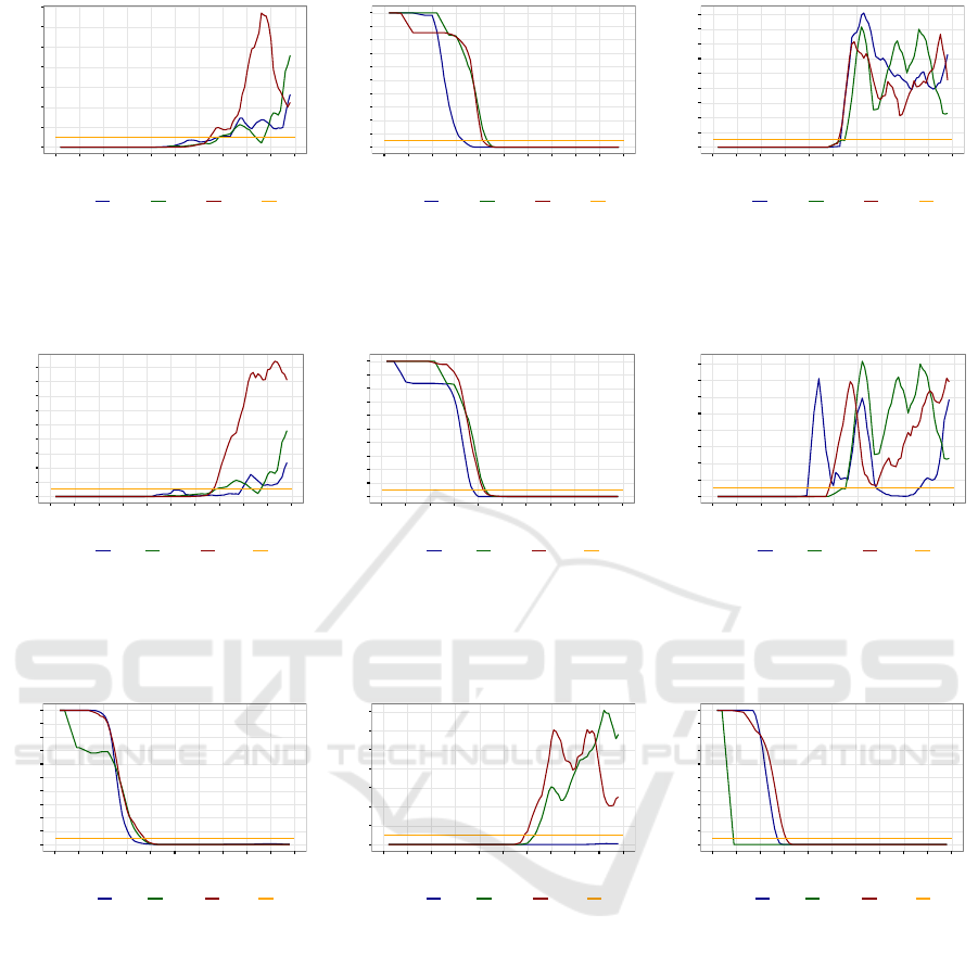
Figure 3. Scenario of Small Enterprise - varying number of edges in G

: betweenness correlation

analysis (a), closeness median analysis (b), closeness correlation analysis (c)

2/3

Figure 4: Scenario of Small Course - varying number of edges in G

: betweenness correlation analysis (a), closeness median

analysis (b), closeness correlation analysis (c).

●● ●● ●● ●● ●● ●● ●● ●● ●● ●● ●● ● ●● ●● ●● ●● ●● ●● ●● ●

●

●● ●● ●● ●● ●● ●● ●● ●● ●● ●● ●● ● ●● ●● ●● ●● ●● ●● ●● ●● ●●

●●

●

●● ●● ●● ●● ●● ●● ●● ●● ●● ●● ●● ● ●● ●● ●● ●● ●● ●● ●● ●● ●● ●● ●● ●● ●● ●● ●● ●● ●

●

0.0

0.1

0.2

0.3

0.4

0.5

0.6

0.7

0.8

0.9

0% 10% 20% 30% 40% 50% 60% 70% 80% 90% 100%

growth

betweenness − spearman.test

config:

● ● ● ●

SE:low SE:mod. SE:high 5%

●● ●●

●

●● ●● ●● ●● ●●

●

●● ●● ●● ●● ●● ●● ●● ●● ●● ●● ●● ● ●● ●● ●● ●● ●● ●● ●● ●● ●● ●● ●● ●● ●● ●● ●● ●● ● ●● ●

●● ●● ●● ●● ●● ●● ●● ●● ●● ●● ●

●

●● ●● ●● ●● ●● ●● ●● ●● ●● ●● ●● ● ●● ●● ●● ●● ●● ●● ●● ●● ●● ●● ●● ●● ●

●● ●● ●● ●● ●● ●● ●● ●● ●●

●

●● ●

●

●● ●● ●● ●● ●● ●● ●● ●● ●● ●● ●● ● ●● ●● ●● ●● ●● ●● ●● ●● ●● ●● ●● ●●

0.0

0.1

0.2

0.3

0.4

0.5

0.6

0.7

0.8

0.9

1.0

0% 10% 20% 30% 40% 50% 60% 70% 80% 90% 100%

growth

closeness − wilcox.test

config:

● ● ● ●

SE:low SE:mod. SE:high 5%

●● ●● ●● ●● ●● ●● ●● ●● ●● ●● ●● ● ●● ●● ●● ●● ●● ●

●

●● ●● ●● ●● ●● ●● ●● ●● ●● ●● ●● ● ●● ●● ●● ●● ●● ●● ●● ●● ●●

●

●● ●● ●● ●● ●● ●● ●● ●● ●● ●● ●● ● ●● ●● ●● ●● ●● ●● ●● ●● ●● ●● ●● ●

●

0.0

0.1

0.2

0.3

0.4

0.5

0.6

0.7

0.8

0% 10% 20% 30% 40% 50% 60% 70% 80% 90% 100%

growth

closeness − spearman.test

config:

● ● ● ●

SE:low SE:mod. SE:high 5%

(a)(b)(c)

Figure 4. Scenario of Small Enterprise - varying number of groups in G

: betweenness correlation

analysis (a), closeness median analysis (b), closeness correlation analysis (c)

●● ●● ●● ●● ●● ●● ●●

●

●● ●●

●

●●

●● ●

●

●●

●

●●

●

●●

●

●● ●

●

●●

●

●● ●

●

●● ●● ●● ●

●● ●●

●

●●

●

●●

●● ●● ●

●

●● ●●

●●

●

●●

●

●●

●

●● ●

●

●● ●● ●● ●● ●● ●● ●

●

●● ●● ●● ●● ●● ●● ●● ●●

●● ●● ●● ●●

●● ●● ●● ●● ●● ●

●● ●

●● ●● ●

0.0

0.1

0.2

0.3

0.4

0.5

0.6

0.7

0.8

0.9

1.0

0% 10% 20% 30% 40% 50% 60% 70% 80% 90% 100%

growth

betweenness − wilcox.test

config:

● ● ● ●

ME:low ME:mod. ME:high 5%

●●

●

●● ●

●●

●

●●

●

●●

●

●● ●● ●● ●● ●● ●● ●● ●● ●● ●● ●● ● ●● ●● ●● ●● ●● ●● ●● ●● ●● ●● ●● ●● ●● ●● ●

●

●● ●● ●● ●● ●● ●● ●● ●● ●● ●● ●● ● ●● ●● ●● ●● ●● ●● ●● ●● ●● ●● ●● ●● ●● ●

●

0.0

0.1

0.2

0.3

0.4

0.5

0.6

0.7

0% 10% 20% 30% 40% 50% 60% 70% 80% 90% 100%

growth

betweenness − spearman.test

config:

● ● ● ●

ME:low ME:mod. ME:high 5%

●● ●● ●● ●● ●● ●● ●●

●

●● ●● ●● ●● ●● ●● ●● ●● ●● ●● ●● ● ●● ●● ●● ●● ●● ●● ●● ●● ●● ●● ●● ●● ●● ●● ●● ●● ● ●● ●● ●● ●● ●● ●●

●

●● ●● ●● ●● ●● ●● ●● ●● ●● ●● ●● ● ●● ●● ●● ●● ●● ●● ●● ●● ●● ●● ●● ●● ●● ●● ●● ●● ● ●● ●● ●● ●● ●● ●● ●● ●● ●● ●● ●● ●● ●● ●● ●● ●● ● ●

●

●● ●● ●

●

●● ●● ●● ●● ●● ●● ●● ●● ●● ●● ●● ● ●● ●● ●● ●● ●● ●● ●● ●● ●● ●● ●● ●● ●● ●● ●● ●● ● ●● ●● ●● ●●

0.0

0.1

0.2

0.3

0.4

0.5

0.6

0.7

0.8

0.9

1.0

0% 10% 20% 30% 40% 50% 60% 70% 80% 90% 100%

growth

closeness − wilcox.test

config:

● ● ● ●

ME:low ME:mod. ME:high 5%

(a)(b)(c)

Figure 5.

Scenario of Medium Enterprise - varying both number of groups in

and number of edges in

: betweenness median analysis (a), betweenness correlation analysis (b), closeness median analysis (c)

3/3

Figure 5: Scenario of Small Course - varying number of groups in G

: betweenness correlation analysis (a), closeness median

analysis (b), closeness correlation analysis (c).

●● ●● ●● ●● ●● ●● ●● ●● ●● ●● ●● ●● ●● ●● ● ●● ●● ●● ●● ●

●

●● ●● ●● ●● ●● ●● ●● ●● ●● ●● ●● ●● ●● ●● ● ●● ●● ●● ●● ●● ●●

●●

●

●● ●● ●● ●● ●● ●● ●● ●● ●● ●● ●● ●● ●● ●● ● ●● ●● ●● ●● ●● ●● ●● ●● ●● ●● ●● ●● ●● ●

●

0.0

0.1

0.2

0.3

0.4

0.5

0.6

0.7

0.8

0.9

0% 10% 20% 30% 40% 50% 60% 70% 80% 90% 100%

growth

betweenness − spearman.test

config:

● ● ● ●

SE:low SE:mod. SE:high 5%

●● ●●

●

●● ●● ●● ●● ●●

●

●● ●● ●● ●● ●● ●● ●● ●● ●● ●● ●● ●● ●● ●● ● ●● ●● ●● ●● ●● ●● ●● ●● ●● ●● ●● ●● ●● ●● ●●

●● ●● ●● ●● ●● ●● ●● ●● ●● ●● ●

●

●● ●● ●● ●● ●● ●● ●● ●● ●● ●● ●● ●● ●● ●● ● ●● ●● ●● ●● ●● ●● ●● ●● ●● ●

●● ●● ●● ●● ●● ●● ●● ●● ●●

●

●● ●

●

●● ●● ●● ●● ●● ●● ●● ●● ●● ●● ●● ●● ●● ●● ● ●● ●● ●● ●● ●● ●● ●● ●● ●●

0.0

0.1

0.2

0.3

0.4

0.5

0.6

0.7

0.8

0.9

1.0

0% 10% 20% 30% 40% 50% 60% 70% 80% 90% 100%

growth

closeness − wilcox.test

config:

● ● ● ●

SE:low SE:mod. SE:high 5%

●● ●● ●● ●● ●● ●● ●● ●● ●● ●● ●● ●● ●● ●● ● ●● ●● ●

●

●● ●● ●● ●● ●● ●● ●● ●● ●● ●● ●● ●● ●● ●● ● ●● ●● ●● ●● ●● ●●

●

●● ●● ●● ●● ●● ●● ●● ●● ●● ●● ●● ●● ●● ●● ● ●● ●● ●● ●● ●● ●● ●● ●● ●

●

0.0

0.1

0.2

0.3

0.4

0.5

0.6

0.7

0.8

0% 10% 20% 30% 40% 50% 60% 70% 80% 90% 100%

growth

closeness − spearman.test

config:

● ● ● ●

SE:low SE:mod. SE:high 5%

(a)(b)(c)

Figure 4. Scenario of Small Enterprise - varying number of groups in G

: betweenness correlation

analysis (a), closeness median analysis (b), closeness correlation analysis (c)

●● ●● ●● ●● ●● ●● ●●

●

●● ●●

●

●●

●● ●

●

●●

●

●●

●

●●

●

●● ●

●

●●

●

●● ●

●

●● ●● ●● ●

●● ●●

●

●●

●

●●

●● ●● ●

●

●● ●●

●●

●

●●

●

●●

●

●● ●

●

●● ●● ●● ●● ●● ●● ●

●

●● ●● ●● ●● ●● ●● ●● ●●

●● ●● ●● ●●

●● ●● ●● ●● ●● ●

●● ●

●● ●● ●

0.0

0.1

0.2

0.3

0.4

0.5

0.6

0.7

0.8

0.9

1.0

0% 10% 20% 30% 40% 50% 60% 70% 80% 90% 100%

growth

betweenness − wilcox.test

config:

● ● ● ●

ME:low ME:mod. ME:high 5%

●● ●● ●● ●● ●● ●● ●● ●● ●● ●● ●● ●● ●● ●● ● ●● ●● ●● ●● ●● ●● ●● ●● ●● ●● ●● ●● ●● ●● ●●

●●

●

●● ●

●●

●

●●

●

●●

●

●● ●● ●● ●● ●● ●● ●● ●● ●● ●● ●● ●● ●● ●● ● ●● ●● ●● ●● ●● ●● ●● ●● ●● ●● ●● ●

●

●● ●● ●● ●● ●● ●● ●● ●● ●● ●● ●● ●● ●● ●● ● ●● ●● ●● ●● ●● ●● ●● ●● ●● ●● ●

●

0.0

0.1

0.2

0.3

0.4

0.5

0.6

0.7

0% 10% 20% 30% 40% 50% 60% 70% 80% 90% 100%

growth

betweenness − spearman.test

config:

● ● ● ●

ME:low ME:mod. ME:high 5%

●● ●● ●● ●● ●● ●● ●●

●

●● ●● ●● ●● ●● ●● ●● ●● ●● ●● ●● ●● ●● ●● ● ●● ●● ●● ●● ●● ●● ●● ●● ●● ●● ●● ●● ●● ●● ●● ●● ●● ●● ●● ●

●

●● ●● ●● ●● ●● ●● ●● ●● ●● ●● ●● ●● ●● ●● ● ●● ●● ●● ●● ●● ●● ●● ●● ●● ●● ●● ●● ●● ●● ●● ●● ●● ●● ●● ●● ●● ●● ● ●● ●● ●● ●● ●● ●● ●● ●●

●

●● ●● ●

●

●● ●● ●● ●● ●● ●● ●● ●● ●● ●● ●● ●● ●● ●● ● ●● ●● ●● ●● ●● ●● ●● ●● ●● ●● ●● ●● ●● ●● ●● ●● ●● ●

0.0

0.1

0.2

0.3

0.4

0.5

0.6

0.7

0.8

0.9

1.0

0% 10% 20% 30% 40% 50% 60% 70% 80% 90% 100%

growth

closeness − wilcox.test

config:

● ● ● ●

ME:low ME:mod. ME:high 5%

(a)(b)(c)

Figure 5.

Scenario of Medium Enterprise - varying both number of groups in

and number of edges in

: betweenness median analysis (a), betweenness correlation analysis (b), closeness median analysis (c)

3/3

Figure 6: Scenario of Medium Course - varying both number of groups in G

and number of edges in G

: betweenness median

analysis (a), betweenness correlation analysis (b), closeness median analysis (c).

and G

= v

= 10, k

= 2, e

= e

= 10).

Figures 2(a) and 2(b) are respectively examples of the

CCT and the NCT graphs produced by Algorithm 4

according to this small setup. Figure 2(c) presents

the produced mixed graph (G

) from both G

and G

using Algorithm 2.

In the example, Figure 2(a) simulates communica-

tions that occur through CCT inside a small course. In

this case, we assume that the course has two groups.

It is possible to view some clusters of communication,

which can be found among students who share a close

relationship, such as work on related tasks, where the

internal processes of the course make them to have

a direct communication. Despite these clusters, it is

possible to observe that the graph is connected. This

means that with the mediation of one or more persons,

the information can be disseminated through the net-

work. In a small network like G

, we can visually

inspect the characteristics that are part of the goals

of our analysis, such as connectivity, the presence of

clusters, and center points connecting them which are

the students identiﬁed as 2 and 7. Clusters commu-

CSEDU 2018 - 10th International Conference on Computer Supported Education

150

Algorithm 4: Synthetic dataset production.

1: function SyntheticDatasets(k,v,e,e

)

2: for all i ← 1 to k do

3: G

← new ScaleFreeGraph(v, e)

4: G

← G

∪G

5: end for

6: for i ← 1 to k

−1 do

7: for j ← i + 1 to k

8: e

← connect(G

)

9: E

← E

∪e

10: end for

11: end for

12: v

← v ·k

13: v

← v

14: G

← new ScaleFreeGraph(v

)

15: return ({G

})

16: end function

Table 2: LP Scenarios.

Scenario Description

SC (G

scale)

= 30, k

= 3, e

= 60

small : e

= 25

medium : e

= 45

large : e

= 55

SC (G

groups)

= 30, e

= 60, e

= 45

low : k

= 2

moderated : k

= 3

high : k

= 5

MC (G

groups)

= 150, e

= 60

low : k

= 10, e

= 120

moderated : k

= 15, e

= 180

high : k

= 25, e

= 300

nicate with each other through the central points. We

applied a similar procedure to produce the graph as-

sociated to the NCT (G

) depicted in Figure 2(b) and

described in Algorithm 4.

Figure 2 explores different network growth (δ) of

the new tool (G

) using ratios such as 25%, 50%,

75%, and 100% in Algorithm 5. It is possible to ob-

serve that both the number of edges in G

and their

weights are explored in different growth ratios (G

25%

(b), G

50%

(d), G

75%

(e), and G

100%

(f)). This leads to

different mixed graphs G

: G

25%

(c), G

50%

(g), G

75%

(h), and G

100%

(i) by mixing G

with G

. By visually

inspecting the instance of G

presented in Figure 2, it

seems that the hierarchical structure does not restrict

the communication ﬂow as the growth ratio of G

in-

creases.

Algorithm 5: Network Growth.

1: function NetGrowth(w

,r)

2: RS ←{}

3: for all δ ← 0 to 100 step r do

4: w

n,δ

← Filter(δ,

100

·w

)

5: w

m,δ

← fMix(w

, w

n,δ

)

6: RS ←RS ∪ f Analyze(w

m,δ

)

7: end for

8: plotCharts(RS)

9: end function

To better comprehend the toy sample, Figure 3

presents descriptive statistics for G

produced by

mixing G

= 10,k

= 2,e

= 10) with G

10,e

= 10). Figure 3(a) depicts the frequency of

degree of G

as G

grows. The degree of vertices

increases as G

grows. The plots in log x log scale

ﬁts a power law distributions, i.e., suggesting a scale-

free graph. This behavior is also summarized in Fi-

gure 3(b). Additionally, Figures 3(c) and 3(d) des-

cribe the closeness and betweenness centrality distri-

bution. In Figure 3(d), the box plot for growth ratios

of 50%, does not present any intersection with box

plots of smaller growth ratios (0% and 25%). This

indicates signiﬁcant difference among them, i.e., the

median closeness of G

50%

is higher than in G

. Ne-

vertheless, the betweenness described in Figure 3(c)

does not present any signiﬁcant difference among

them.

Furthermore, Figures 3(e) and 3(f) present, re-

spectively, a scatter plot for the closeness and bet-

weenness correlation between G

and G

. The cor-

relation is plotted with a conﬁdence interval of 95%.

It is possible to observe that both are correlated. This

indicates, for example, that although Figure 3(c) indi-

cates an increase in closeness introduced by G

, such

an increase does not change the topology of G

, i.e., it

is not introducing a complementary behavior. It is ac-

tually just introducing an increase in the scale of G

with respect to G

However, analyzing these plots may not be appli-

cable in general, especially for more extensive net-

works, such as in a distance learning education. To

tackle this problem, the MGF uses statistical analysis

to assess and monitor the complementarity of NCT. It

applies the Wilcoxon rank sum test and the Spearman

rank correlation test to both betweenness and close-

ness as described in our Main Analysis.

5.4 Sensitive Analysis

In this section, we evaluate the proposed MGF using

synthetic data described in Section 5.1. It is worth

Evaluating the Complementarity of Communication Tools for Learning Platforms

151

mentioning that the objective of this section is not to

assess the impacts of introducing a NCT. Instead, we

intend to evaluate whether the MGF can distinguish

and G

according to the inﬂuence of G

. We have

conducted a sensitivity analysis between networks.

The goal is to identify if the NCT keeps the communi-

cation ﬂow provided by CCT or if it introduces alter-

native and signiﬁcant changes in the communication

ﬂows.

In the ﬁrst scenario described in Table 2 we explo-

red the number of communication ﬂows in the NCT

of courses under a small, medium, and large scale.

Regarding betweenness, Figure 4(a) indicates a signi-

ﬁcant difference for the correlation, when the growth

ratio is greater than 60%. Additionally, in terms of

closeness, both median (Figure 4(b)) and correlation

(Figure 4(c)) presents a signiﬁcant difference when

the growth ratio are greater than 40% and 55%, re-

spectively.

We also explored the second scenario for cour-

ses, in which we vary the number of groups inside

. Figure 5(a) indicates a signiﬁcant difference for

the betweenness correlation when the growth increa-

ses. They were reached after a growth of 65%. In

fact, the growth threshold for a signiﬁcant difference

occurs later when the group size is moderate or low.

When it comes to closeness, both median analysis (Fi-

gure 5(b)) and correlation analysis (Figure 5(c)) pre-

sent a signiﬁcant differences when growth is greater

than 40%. This is interesting as it indicates an incre-

ase in the number of messages in G

and a difference

in the network communication topology, as well.

In our third evaluation scenario, we explored the

number of communication ﬂows in the NCT and the

number of groups inside G

of a Medium Course un-

der small, medium, and large scale. Regarding be-

tweenness, as depicted in Figures 6(a) and 6(b), we

observe a signiﬁcant difference for the median and

correlation as the growth ratio reaches 35% and 60%,

respectively. A similar behavior occurs with close-

ness. Figure 6(c) indicates a signiﬁcant difference for

the closeness median when the growth is greater than

35%. In fact, for the medium size case, only when re-

aching an increase higher than 70% we found a clear

signiﬁcant difference. Before this value, we observed

an oscillatory behavior around the signiﬁcance thres-

hold.

6 CONCLUSION

This paper proposes a Mixed Graph Framework

(MGF), which aims at providing a set of quantita-

tive approaches to analyze the complementary of a

new communication tool (NCT) with relation to a cur-

rent communication tool (CCT) in a learning platform

(LP). This is done by measuring when the NCT brings

signiﬁcant differences in the overall educational com-

munication ﬂow concerning the usage of the CCT.

We model CCT and NCT communication interacti-

ons as the weighted graphs G

and G

, respectively.

From these graphs, the MGF computes a mixed graph

) that combines both G

and G

considering their

usage. Our approach is then able to identify changes

in overall communication within the educational.

We also evaluated the proposed MGF using synt-

hetic data from which we have conducted a sensi-

tive analysis. The sensitivity analysis is used to com-

pare the weighted closeness and betweenness of both

and G

. Our approach can identify whether G

is providing any changes in the entire communica-

tion ﬂow. It is worth mentioning that our method

does not propose adopting the NCT as a replacement

for the CCT to promote communication empower-

ment. Instead, the goal of MGF is to aid managers in

a decision-making process, giving them elements to

conduct what-if analysis while deploying NCTs and

measuring its inﬂuence in the entire set of communi-

cation solutions adopted in the educational.

We considered the evolution of a single network

over time including time notion in the proposed fra-

mework as a promising future research. As well as

performing case studies with networks of different si-

zes, which is a useful analysis for educational institu-

tions with scenarios of reorganizations, mergers and

divisions of courses.

ACKNOWLEDGMENTS

The authors would like to thank CNPq, CAPES, and

FAPERJ for partially funding this research.

REFERENCES

Ahuja, R. K., Magnanti, T. L., and Orlin, J. B. (1993). Net-

work Flows: Theory, Algorithms, and Applications.

Pearson, Englewood Cliffs, N.J, 1 edition edition.

Barab

asi, A.-L. and Albert, R. (1999). Emergence of sca-

ling in random networks. Science, 286(5439):509–

512.

Benevenuto, F., Rodrigues, T., Cha, M., and Almeida, V.

(2009). Characterizing user behavior in online social

networks. In Proceedings of the ACM SIGCOMM In-

ternet Measurement Conference, IMC, pages 49–62.

Cadima, R., Ferreira, C., Monguet, J., Ojeda, J., and Fer-

nandez, J. (2010). Promoting social network aware-

CSEDU 2018 - 10th International Conference on Computer Supported Education

152

ness: A social network monitoring system. Computers

and Education, 54(4):1233–1240.

Chai, S. and Kim, M. (2012). A socio-technical approach to

knowledge contribution behavior: An empirical inves-

tigation of social networking sites users. International

Journal of Information Management, 32(2):118–126.

Chatti, M., Jarke, M., and Frosch-Wilke, D. (2007). The

future of e-learning: a shift to knowledge networking

and social software. International Journal of Know-

ledge and Learning, 3(4-5):404–420.

Dalgaard, P. (2008). Introductory Statistics with R. Sprin-

ger, New York, 2nd edition edition.

Devore, J. L. and Berk, K. N. (2011). Modern Mathemati-

cal Statistics with Applications. Springer, New York ;

London, 2nd ed. 2012 edition edition.

Hamulic, I. and Bijedic, N. (2009). Social network analy-

sis in virtual learning community at faculty of infor-

mation technologies (ﬁt), Mostar. In Procedia - So-

cial and Behavioral Sciences, volume 1, pages 2269–

2273.

Hrastinski, S. (2009). A theory of online learning as online

participation. Computers and Education, 52(1):78–

82.

Kellogg, S., Booth, S., and Oliver, K. (2014). A so-

cial network perspective on peer supported learning in

MOOCs for educators. International Review of Rese-

arch in Open and Distance Learning, 15(5):263–289.

Kleinberg, J. (1999). Authoritative sources in a hyperlinked

environment. Journal of the ACM, 46(5):604–632.

Kolaczyk, E. D. (2009). Statistical Analysis of Network

Data: Methods and Models. Springer, New York,

2009 edition edition.

Larsen, R. J. and Marx, M. L. (2005). An Introduction to

Mathematical Statistics and Its Applications. Prentice

Hall, Upper Saddle River, N.J, 4 edition edition.

Mazzolini, M. and Maddison, S. (2003). Sage, guide or

ghost? the effect of instructor intervention on student

participation in online discussion forums. Computers

and Education, 40(3):237–253.

Moore, J., Dickson-Deane, C., and Galyen, K. (2011). E-

Learning, online learning, and distance learning envi-

ronments: Are they the same? Internet and Higher

Education, 14(2):129–135.

Nettleton, D. (2013). Data mining of social networks repre-

sented as graphs. Computer Science Review, 7(1):1–

34.

Newman, M. (2003). The structure and function of complex

networks. SIAM Review, 45(2):167–256.

Newman, M., Watts, D., and Strogatz, S. (2002). Random

graph models of social networks. Proceedings of the

National Academy of Sciences of the United States of

America, 99(SUPPL. 1):2566–2572.

Ngai, E., Tao, S., and Moon, K. (2015). Social media re-

search: Theories, constructs, and conceptual frame-

works. International Journal of Information Manage-

ment, 35(1):33–44.

Opsahl, T., Agneessens, F., and Skvoretz, J. (2010). Node

centrality in weighted networks: Generalizing degree

and shortest paths. Social Networks, 32(3):245–251.

Prado, A. and Baranauskas, M. (2013). Addressing structu-

ral and dynamic features of scientiﬁc social networks

through the lens of Actor-Network Theory. Social

Network Analysis and Mining, 3(4):1263–1276.

Siribaddana, P. (2014). Making distance learning an ef-

fective health information systems training strategy:

A combined social network analysis and content ana-

lysis perspective. Electronic Journal of Information

Systems in Developing Countries, 61(1).

Wasko, M., Teigland, R., and Faraj, S. (2009). The provi-

sion of online public goods: Examining social struc-

ture in an electronic network of practice. Decision

Support Systems, 47(3):254–265.

Wasserman, S. and Faust, K. (1994). Social Network Analy-

sis: Methods and Applications. Cambridge University

Press, Cambridge ; New York, 1 edition edition.

Evaluating the Complementarity of Communication Tools for Learning Platforms

153