Proposed Solutions to the Tripper Car Positioning Problem

Felipe Novaes Caldas

and Alexandre Xavier Martins

Gerência de Automação, Vale, São Gonçalo do Rio Abaixo, MG, Brazil

Instituto de Ciências Exatas e Aplicadas, Universidade Federal de Ouro Preto, João Monlevade, MG, Brazil

Keywords:

Tripper Car, Combinatorial Optimization, Dynamic Programming.

Abstract:

The trippers are equipments often found in mineral processing plants. Their role is to distribute ore coming

from past stages of process in a silo with several hoppers. Positioning trippers is a scheduling problem deﬁned

by position determination of the equipment through the bins and along time. The system silo-tripper was

modeled as a combinatorial linear optimization program aiming to get the optimal tripper positioning. Two

paradigms were used to ﬁnd out an exact solution: mixed integer linear programming and dynamic program-

ming.

1 INTRODUCTION

Storage silos are structures designed to store bulk so-

lid materials. Its function is to form an intermediary

stock between two stages of the mineral processing

cycle. Conveyor belts fulﬁll the role of bringing the

ore from an earlier stage and storing it there. After-

wards, this material is removed by equipments called

feeders, located right below each one of these cham-

bers, proceeding with the mineral processing task

(Wills and Napier-Munn, 2015). The number of fee-

ders required in an intermediate storage silo design is

proportional to the ore volume that will be handled.

In this way, a silo must be subdivided into smaller

chambers, according to the number of feeders requi-

red, providing an individualized area for the installa-

tion of each one of these equipments under the struc-

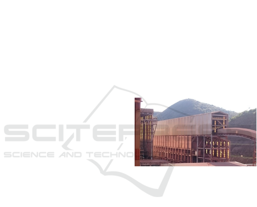
ture of the storage silo (Gupta and Yan, 2006). The

vertical pillars that are observed along the lower struc-

ture of the building, as shown in Figure 1, indicate the

approximated location of the subdivisions. The area

deﬁned by two pillars and ﬁlled by a concrete wall is

the region where a chamber or bin of the silo is deﬁ-

ned. In this example, there are sixteen subdivisions.

In the right side of the image, there is a structure that

projects over the front wall of the silo, it is called a

conveyor belt. Its role is to carry ore coming from an

earlier stage of the process to the storage silo.

A tripper is a car designed to distribute ore along

the top opening of a storage silo (Wills and Napier-

Munn, 2015). This equipment is constituted by a mo-

bile metallic structure that physically supports a dis-

Figure 1: Example of storage silo from Brucutu mine –

Vale.

charge point of the conveyor belt. The car is driven by

steel wheels located under its structure. Metallic rails

support and guide the tripper longitudinally along the

silo, allowing the ore carried by the conveyor belt to

be conveniently distributed between all subdivisions

(Swinderman, 2014).

An example of tripper can be seen in Figure 2.

This equipment is located over the silo SL-133A-

9101 at the processing plant from Brucutu mine. This

site is an asset belonging to Vale mining company.

The conveyor belt can be seen at the bottom left of

the ﬁgure and runs all over the top of the storage silo.

Its location is identiﬁed by the roller frame structures

mounted along its side. The silo opening is shown

below the conveyor belt and behind the guardrail, the

ore is deposited in this region. The tripper is seen in

the central area of the ﬁgure, over the conveyor belt.

The discharge point extends from the top of the equip-

ment and continues until reach the silo opening. One

344

Novaes Caldas, F. and Xavier Martins, A.

Proposed Solutions to the Tripper Car Positioning Problem.

DOI: 10.5220/0006806303440352

In Proceedings of the 20th International Conference on Enterprise Information Systems (ICEIS 2018), pages 344-352

ISBN: 978-989-758-298-1

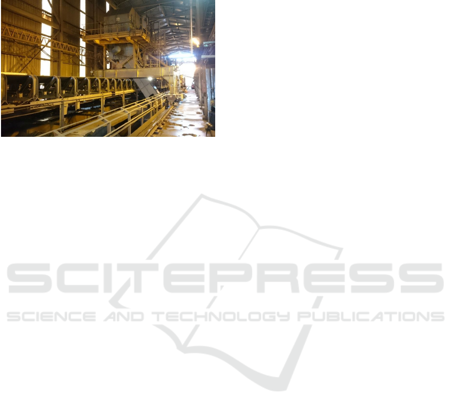
of the car rails is located to the right of the guardrail,

it is supporting the tripper front right wheels.

Figure 2: Example of tripper car from Brucutu mine – Vale.

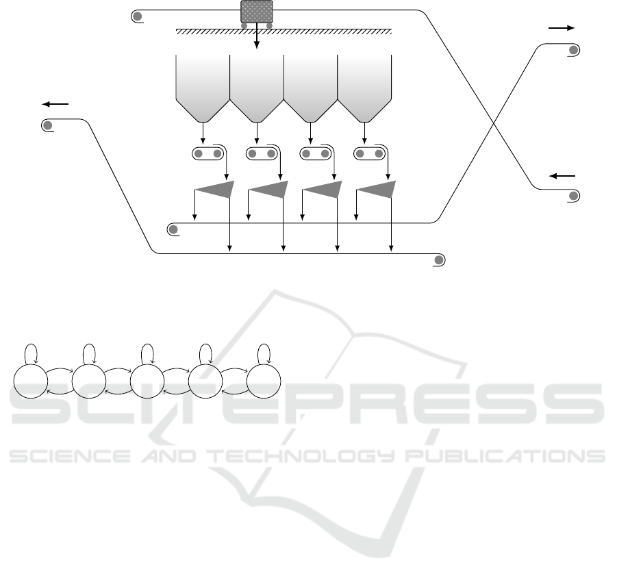
The ﬂowchart shown in Figure 3 provides an il-

lustrative example of a bulk mineral processing. The

system’s feed ﬂow comes from a conveyor belt. The

tripper has the role of distributing this material along

the upper opening of the storage silo. The ore is wit-

hdraw by feeders and directed to sieves. In this stage,

the material is split according to its granulometry, one

part returning to the previous process as by-product 1

and another part proceeds further as by-product 2.

The tripper car movement is controlled by au-

tomation systems. Electric motors attached to the

equipment wheels are driven by this systems (Boyer,

2010) in such way it is possible to position the equip-

ment, deﬁning which silo’s bin will receive the ma-

terial loaded by the conveyor belt. Three actions are

possible through the automation operation interface:

move to the right, move to the left, and halt. The ore

ﬂow isn’t interrupted during the moving process.

Model-based predictive control (MPC) systems

are a class of controllers that deﬁne their control

action outputs based on future predictions of the pro-

cess states. These predictions are performed by dyna-

mic models that represent the behavior of the system

over time, inside a ﬁnite time frame. As an optimizer,

the MPC algorithm uses these informations to build

an optimal control output aiming a desired behavior

for the process. Only the present action of the entire

output forecast window is sent to the plant at each

iteration. In the next run cycle, the entire window

is recalculated and the new control action is formed

(García et al., 1989; Camacho and Bordons, 2007).

This ﬁrst version of MPC was not able to handle

discrete variables, restricting its application to conti-

nuous process. As an evolution of the initial proposal,

the algorithm was expanded to consider discrete vari-

ables, logics and rules, in addition to the continuous

variables that were already considered in the ﬁrst ver-

sion. This expanded form is known as hybrid MPC

(Bemporad and Giorgetti, 2006; Borrelli et al., 2005).

This controller is suitable to deal with the problem of

tripper positioning since this process has both conti-

nuous (level, mass ﬂow) and discrete (position) vari-

ables. A framework based on hybrid MPC was used

by (Karelovic et al., 2015) to solve the tripper positi-

oning problem. The criteria used by the authors to set

up the controller objectives were bins level stabiliza-

tion and minimization of the car movement.

The purpose of this work is to develop a solution

to the tripper positioning problem based directly on

mixed integer linear programming. In this case, the

objective of the control system is to minimize the va-

riations of bins levels, ensuring that these variables

remain stable regarding the process constraints. Fi-

nally, a dynamic programming algorithm is proposed

aiming the reduction of the time required to ﬁnd the

solution of the optimization problem.

2 DEVELOPMENT

The development of the mathematical models that

describe the behavior of the silo-tripper system is the

starting point for the study of the solutions to the pro-

blem of car positioning. The features of the optimi-

zation model, such as instance input data, decision

variables, constraints and objective function, are des-

cribed in detail. This formulation will be solved later

by means of mixed integer linear programming and

dynamic programming.

2.1 Mathematical Model

The Figure 4 presents the moving possibilities of a

n-bins silo. At any position, the equipment can only

move to one of the adjacent places or remain in the

same position over which it is located. For example,

if it’s in p

position then the movement options will

be {p

, p

}. Moving the car to a position not ad-

jacent to the current one implies crossing all the in-

termediate positions between the points of departure

and destination. Consequently, tripper directs the ore

ﬂow to the bin whose position is overlapped by cur-

rent equipment displacement. The choice of feeding

position is a task with temporal dependence since the

movement speed of the equipment is ﬁnite.

There is a risk that the material may eventually

lacks in one of the bins since tripper may only be in

a particular place at any time. This may occur even

in situations where the mass balance of the system

is balanced, that is, the total mass ﬂow fed is equal to

the total withdrawn. To work around this problem, the

tripper must be moved along the bins openings so that

Proposed Solutions to the Tripper Car Positioning Problem

345

tripper

feed

by-product 1

by-product 2

Figure 3: Diagram illustrating a granular ore sifting process. The tripper is represented by a dotted rectangle with two wheels

indicated as small circles. A four-bin silo is shown under the tripper. Below each bin there is a belt feeder. The sieves are

represented by gray triangles. Conveyor belts are signaled by the ore ﬂow they carry: feed, by-product 1 and by-product 2.

. . .

Figure 4: State machine representing the possibilities of

tripper positioning.

the material addition by the conveyor belt does not

allow any lack of ore. It is also needed to limit the bins

levels according to the maximum capacity restrictions

of the silo.

The time required for the tripper to travel through

the region corresponding to the opening of a bin, mo-

ving uninterruptedly, is proportional to the length of

the traveled region and inversely proportional to the

moving speed of the car. In order to simplify the mo-

del, the time elapsed by tripper to cross a whole bin

is considered constant in any situation in which the

silo subdivisions have the same size and the tripper

has constant speed. The forecast time window, over

which the prediction will be performed, is divided

into multiples of this minimum time. The size of this

window deﬁnes the ﬁrst dimension of the positioning

problem model.

The second problem dimension is deﬁned by the

set P of feasible positions for the tripper, whose num-

ber of elements corresponds to the number of bins.

The positioning scheduling is deﬁned as the choice

of a sequence of car movement actions along a ﬁnite

window of future time. The purpose of these acti-

ons is to keep the variables controlled within the ope-

rational constraints established for the problem. The

future time window is mapped to a ﬁnite set T , com-

posed of the current state of the system added by t − 1

future steps. These extra iterations are necessary to

make the model able to predict in advance the out-

come of the control actions that will be taken over

time, verifying if the established constraints will be

violated at some point.

The Figure 5 shows a graph of the model, deve-

loped to represent a tripper positioning problem. The

initial positions, relative to the time t

, are contained

in the set {p

∈ N | 1 ≤ i ≤ n}, being n the num-

ber of bins. From any initial position, the subsequent

positions are chosen at each iteration, regarding the

movement constraints over which the possible positi-

ons are limited the current position and adjacent ones.

Finally, the possible positions in the ﬁnal step t

are

contained in the set {p

∈ N | 1 ≤ i ≤ n}.

Therefore, the parameters deﬁning the size of an

instance are:

• Number of bins: n;

• Prediction window size: t.

2.1.1 Instance Parameters

The instance parameters are presented in the Table 1.

In this work, the input rates q and output set Q are de-

ﬁned as constants throughout all steps. However, this

parameters may be easily transformed to have multi-

ple different values through time.

The instance size is deﬁned by the sets T periods

ICEIS 2018 - 20th International Conference on Enterprise Information Systems

346

. . .

Figure 5: Graph representing the positioning possibilities of

a tripper throughout iterations.

of time and P bins. The initial level of each one of

the bins is deﬁned by the vector L

. The levels values

are constrained between l

min

and l

max

. The starting

position of the tripper car is deﬁned by p. The silo

emptying rate is deﬁned as K. This parameter deﬁnes

the amount of ore that each one of the bins is capable

of storing according to the dynamic equation of the

process.

2.1.2 Decision Variables

The decision variables are presented in the Table 2.

The most important of them is the matrix I that repre-

sents the tripper positions through time. It is a set of

binary values that deﬁnes the car positioning over n

possible positions along t steps (Wolsey, 1998).

The states of the P bins levels along the T iterati-

ons are deﬁned by L. The matrices A and B represent

slack variables for bins levels. The Z set represents

the auxiliary variables for the MinMax cost function.

Table 1: Instance parameters.

Parameter Description

T Periods set

P Bins set

n Number of bins

t Number of periods

Inicial level

max

Maximum level

min

Minimum level

q Input mass ﬂow

Q Output mass ﬂow

K Bins level coefﬁcient

p Initial position

Table 2: Decision variables.

Variable Description

I Tripper positions

A Low level slack

B High level slack

L Levels

Z MinMax auxiliary

2.1.3 Constraints

The dynamic equation that deﬁnes the level of a bin i

along time is shown by Equation 1 (Pal et al., 2014):

= K

− Q

)dt (1)

Being L

the level of some bin, K

the bin volume coef-

ﬁcient and Q

the mass ﬂow of the tripper and Q

an individual feeder.

The Equation 13 deﬁnes the mass accumulation at

each period of time based on Equation 1, adding the

slack variable components. At each step, the bin loca-

ted under the current tripper position is increased by

the mass ﬂow input q. The initial level is deﬁned by

Equation 8. This constraint represents the available

ore mass in the bin at ﬁrst period of time.

If the Equation 1 is not balanced, for example, the

input mass rate is different from the mass output rate,

the bin may empty or ﬁll up completely occasionally

in any of the solution steps. Two slack variables sets

A and B have been added to ensure that the problem

becomes feasible with any instance parameters. The

ﬁrst handle bin level below l

min

, as deﬁned in Equati-

ons 11 and 12, and the second handle bin level above

max

, as shown by Equations 9 and 10.

The tripper starting position is deﬁned by parame-

ter p in Equation 7. The Equation 3 determines that

the car may be only on a single bin at each iteration.

The moving rules along the periods of time are deﬁ-

ned by the Equation 4. It deﬁnes that the car posi-

tion in a given iteration is only feasible if the tripper

is kept at the same place or moves to a immediately

adjacent position. The Equations 5 and 6 determine

the moving rules if the equipment is in the ﬁrst or last

position over the silo.

Proposed Solutions to the Tripper Car Positioning Problem

347

≤ L

i, j

, ∀ j ∈ T, i ∈ P (2)

∑

i∈P

i j

= 1, ∀ j ∈ T (3)

i, j

≤ I

i−1, j−1

+ I

i,i−1

+ I

i+1, j−1

, (4)

∀ i ∈ [2, n − 1], j ∈ [2, t]

1, j

≤ I

1, j−1

+ I

2, j−1

, ∀ j ∈ [2,t] (5)

n, j

≤ I

n, j−1

+ I

n−1, j−1

, ∀ j ∈ [2,t] (6)

p,1

= p (7)

i,1

= L

, ∀ i ∈ T (8)

i, j

= ∆A

i, j

+ A

i−1, j

, ∀ i ∈ P, j ∈ T (9)

∆A

i,1

= 0, ∀ i ∈ V (10)

i, j

= ∆B

i, j

+ B

i−1, j

, ∀ i ∈ P, j ∈ T (11)

∆B

i,1

= 0, ∀ i ∈ V (12)

i, j+1

= L

i, j

+ K

(q · I

i, j

− Q

) + ∆A

i, j+1

(13)

− ∆B

i, j+1

, ∀ i ∈ P, j ∈ [1,t − 1]

i, j

≤ l

max

, ∀ i ∈ P, j ∈ T (14)

i, j

≥ l

min

, ∀ i ∈ P, j ∈ T (15)

2.1.4 Objective Function

The objective function is based on the principle Min-

Max (Rich and Knight, 1991). Its purpose is to max-

imize the lowest level value between all bins at each

period, not allowing ore to lack in any bin at no time.

The Z set, as shown by Equation 2, is deﬁned as the

lowest value of the bins levels reached on each step.

The solution is found by maximizing the result of Z

set summation. The cost function for the problem can

be seen in Equation 16:

Maximize

∑

j∈T

−

∑

i∈P, j∈T

i j

−

∑

i∈P, j∈T

i j

(16)

s.t. Z

≤ L

i, j

, ∀ j ∈ T, i ∈ P

2.2 Mixed Integer Linear Programming

The mixed integer linear programming is a mathema-

tical method whose purpose is to ﬁnd the best solution

for a cost function within a set of constraints deﬁned

by linear relations. The variables handled by this for-

mulation can be represented as either continuous or

integer values(Papadimitriou and Steiglitz, 1998).

Two solvers are used to deal with the proposed

model for the tripper positioning problem. The ﬁrst

one is the Glpk (GNU Linear Programming Kit). The

second choice is IBM’s Cplex Optimizer. The ob-

jective is to compare between the outcome of an open

source solver relative to one proprietary system in

task of solving the optimization problem.

2.3 Dynamic Programming

Dynamic programming is a paradigm of computer

science characterized by ﬁnd the solution of a com-

plex problem by solving its smaller subproblems.

Each subproblem is solved only once and the result

is stored in a table to be query later when needed, rat-

her than recursively computing it whenever necessary

(Levitin, 2012; Cormen et al., 2001).

The subproblems of the positioning problem are

deﬁned as the solution of the this problem in each

one of the intermediate steps. This procedure starts

at the ﬁrst iteration goes through incrementally until

reach the last period. Two tables were created to store

the partial result of the subproblems: the ﬁrst handle

cost values and the second handles positions history.

These tables are identiﬁed as Table and P in the Algo-

rithm 1. The variables referenced by this pseudocode

are listed in Tables 1 and 2.

The algorithm ﬁrst step is to update the bins le-

vels L according to the dynamic model of the process

(lines 2 and 3). In the next step, the value of the cost

function c is updated with the lowest level value in the

current iteration (line 4). The variable Table is upda-

ted if there is no cost value related to the current step

recorded in Table or if the current cost is greater than

or equal to the already stored value, then recursion is

continued (line 6). Otherwise, if the current cost is

less than the recorded cost, the function returns im-

mediately. The best possible solution is stored in the

global variable Best in the last step of the tripper po-

sitioning procedure (lines 12 and 14).

Algorithm 1: Dynamic Programming.

1: function SEARCHMAXIMUM(c, L, Q, q, P, p, s)

2: L[p] ← L[p] + q

3: L ← L − Q

4: c ← c + min(L)

5: if Table[s] =

0 or c ≥ Table[s] then

6: Table[s] ← c

7: P[s] ← p

8: if s 6= t then

9: for i ← max(1, p − 1) to min(n, p + 1) do

10: SearchMaximum(c, L, Q, q, i,P, s + 1)

11: end for

12: else

13: if Table[t] < c then

14: Best ← P

15: end if

16: end if

17: end if

18: end function

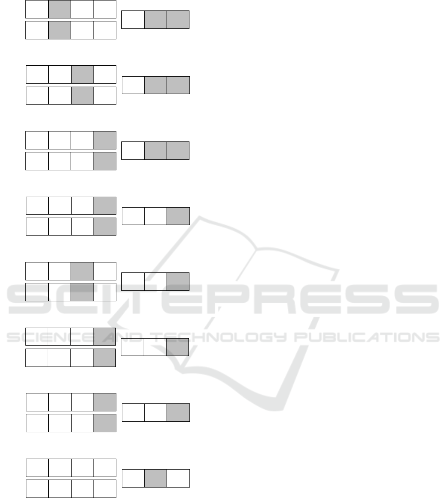
The Figure 6 gives an example of the execution of

the proposed algorithm for instance of three bin silo

and four units time window. Each one of ﬁgures, ran-

ICEIS 2018 - 20th International Conference on Enterprise Information Systems

348

(a)

50 99

1 1

1 2 3 4

52 49 49

1 2 3

(b)

50 99 147

1 1 1

1 2 3 4

54 48 48

1 2 3

(c)

50 99 147 194

1 1 1 1

1 2 3 4

56 47 47

1 2 3

(d)

50 99 147 194

1 1 1 2

1 2 3 4

53 49 47

1 2 3

(e)

50 99 147 194

1 1 2 2

1 2 3 4

51 50 48

1 2 3

(f)

50 99 147 194

1 1 2 1

1 2 3 4

53 49 47

1 2 3

(g)

50 99 147 194

1 1 2 2

1 2 3 4

50 52 47

1 2 3

(h)

50 99 147 194

1 1 2 2

1 2 3 4

50 49 50

1 2 3

Figure 6: Example of eight iterations of dynamic program-

ming algorithm for a silo with three bins.

ging from 5(a) to 5(h), represents one of the algorithm

steps. The two tables on the left side of any subﬁgure

represent Table and P, respectively. The arrow over

them indicates the current period of time and the re-

cursion direction. The left-sided arrow means that the

algorithm execution is returning to a previous step, a

right-arrow indicates that the execution is advancing

to the next step and, ﬁnally, the down arrow shows

that the position is at the same place as it were in last

iteration. A gray ﬁlling color in a cell indicates an

update in its value. The table on the right side of a

subﬁgure represents the current bins levels. An upper

arrow indicates the position and direction of the trip-

per movement. Minimum levels in each period are

indicated by a gray color ﬁlling the respective cells.

The ﬁrst step of execution is shown by Figure 5(a).

The three bins are initialized with 50% level value, the

tripper feed ﬂow rate is set with 3 and the three feeders

ﬂow rate with 1. The ﬁrst action of the car is to remain

at the bin 1. The levels are decremented by one unit

and the bin 1 level is added by 3 units. The bins with

the lowest level value are 2 and 3, they are colored

with gray. The current step cost is the initial cost 50

from the past step added by the minimum step level

value 49, which is the lowest level value. The new

partial cost for this step is 99. This value is stored in

the table along with the position of the car.

This procedure is repeated until there are no new

additions to the table or until the execution of the al-

gorithm reaches the maximum limit of steps t. In this

case, the current solution becomes the new best if its

cost is higher than the cost of the previous best solu-

tion already found so far. A check mark label X is

added to a subﬁgure indicating that a new best solu-

tion was found, as shown in Figure 5(c).

3 RESULTS

Three tests are presented in this section. The ﬁrst one

is a comparison between the control proposal by level

stabilization and minimization of the car movement,

as indicated by (Karelovic et al., 2015), and the algo-

rithm proposed in this work for the positioning pro-

blem. The second test is done over a silo with imba-

lanced ﬂow rates, the purpose is to verify the proposed

model response in this scenario. The last test compa-

res the performance of the Cplex and Glpk resolvers

with respect to the dynamic programming algorithm.

The computational tests were performed over an Intel

Core i5 4570 machine with 16GB of DDR3 memory.

The ﬁrst test was performed over a three-bin silo

instance. The initial levels values were deﬁned as

L = {90, 50, 10}, the feeder ﬂow rates Q = {3, 1, 2},

the tripper feeding ﬂow rate was q = 6 and the starting

position, p = 1. The objective is to compare the two

proposals of silo level control. The stabilization stra-

tegy was adjusted in way to keep bins levels within an

acceptable range of 20% ≤ L ≤ 80%.

Proposed Solutions to the Tripper Car Positioning Problem

349

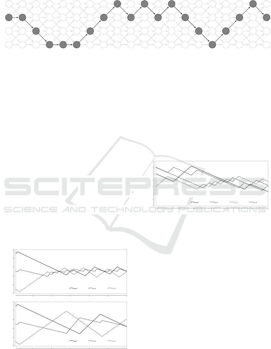
Figure 7: Positioning schedule for a tripper car. This instance is composed by a 4-bin silo with a time window of 20 periods.

The white letter S indicates the starting position.

The Figure 8 shows the test results. The upper

chart shows the behavior of the bins levels values over

time in response to the actions taken by tripper to

maximize the lowest bin level in each iteration. In

this case, after approximately 20 time periods, the le-

vels stabilize within a value range ranging from 40%

to 60%. The test of movement minimization strategy,

as seen in the lower chart of Figure 8, could kept the

bins levels within the requested value range of 20%

and 80%. In this case, the number of car movement

were much smaller than in the ﬁrst strategy, as indi-

cated by the small amount of reversions in the rate of

variation of the levels values.

The test was done considering an instance with

unbalanced loads. The system was set up as a 4-bins

silo, where feed output ﬂow rates were {Q

= 4, ∀ i ∈

P} and input ﬂow rate q = 16, the initial levels were

deﬁned as L = {50, 60, 30, 60}. In this case, there is

a real possibility of material lacking in some of the

bins if the tripper positioning scheduling is done in-

correctly. Figure 7 shows the resulting positioning for

this instance. The white letter S indicates the start

position p = 3. The car is positioned through the 20

10 20 30 40 50 60

100

level (%)

bin 1 bin 2

bin 3

10 20 30 40 50 60

100

periods (t)

level (%)

bin 1 bin 2 bin 3

Figure 8: Comparative tests between the strategies of mo-

vement minimization (top chart) and maximization of the

lowest level at each iteration (bottom chart).

periods in all possible positions in order to maximize

the minimum levels at each period over time.

The imbalance between input and output ﬂow

rates implies in decline of the bins average levels

through time as shown by Figure 9. The initial and

ﬁnal average levels were 50 and 31 conﬁrming the

expected behavior. However, the initial standard de-

viation of bins levels was 14.1 against the ﬁnal value

of 6.6, that is, not only the minimum levels were kept

at higher values but their variabilities was also decre-

ased.

2.5 5 7.5 10 12.5 15 17.5 20

periods(t)

level (%)

bin 1 bin 2 bin 3 bin 4

Figure 9: Results of a test with a 4-bin silo instance in a 20

periods time window.

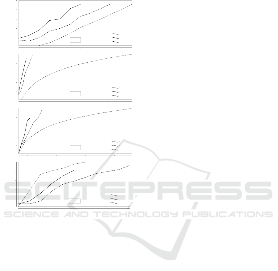
The purpose of the third set of tests is to compare

the performance of the solvers and the dynamic pro-

gramming algorithm. The tests were done in a silo

instance with n ∈ {3, 5,9, 16} bins and with a fore-

cast window of t time periods. These parameters were

varied exhaustively within a time range of 1000 se-

conds, to verify the response time of the solvers. The

parameters of ﬂow rates chosen for the feeders were

= 1, ∀i ∈ P}, the feed ﬂow rate of the tripper was

q = n and the starting position was p = 1. It is ex-

pected that the time elapsed to solve an instance is

proportional to the number of bins n. This variable

represents one of the problem sizes, along to the time

periods t, and its increase is directly related to an in-

crease of the problem complexity.

The Figure 10 displays the tests results. The dyn-

amic programming algorithm was asymptotically fas-

ter in tests with the number of bins n ∈ {3, 5,9}. The

sharp discrepancy between the result of DP regarding

to the results of solvers in the tests with n ∈ {5, 9}

ICEIS 2018 - 20th International Conference on Enterprise Information Systems

350

n = 3

10 20 30 40 50 60

0.1

100

1,000

elapsed time (s)

Glpk

Cplex

n = 5

100 200 300

0.1

100

1,000

elapsed time (s)

Glpk

Cplex

n = 9

25 50 75 100 125 150 175 200

0.1

100

1,000

elapsed time (s)

Glpk

Cplex

n = 16

10 20 30 40 50 60

0.1

100

1,000

periods (t)

elapsed time (s)

Glpk

Cplex

Figure 10: Tests results of Cplex and Glpk solvers and dyn-

amic programming algorithm.

suggests that in these cases the dynamic programming

has order of complexity lower than the algorithms of

mixed integer linear programming. With n = 16 the

two solvers results were superior to the proposed al-

gorithm. At n = 3, although DP performance was fas-

ter than the other methods, it was asymptotically si-

milar. One theory to explain this behavior is that the

algorithm could not take advantage of higher level of

symmetry in a n = 3 instance. Cplex was faster than

Glpk in all instances tested. One point in favor of

the dynamic programming algorithm is the fact that

Cplex is able to handle multiple threads (were four in

this scenario) boosting performance of solving pro-

cess. While current implementation of the proposed

solution presented in this work can just handle one

thread at time.

4 CONCLUSION

This work proposes a new approach to solve the trip-

per positioning problem. The objective was to model

the silo-tripper system as a combinatorial optimiza-

tion problem and solve it by means of exact methods

directly, without the use of hybrid MPC frameworks.

The proposal was to maximize the lowest bin level

of the silo in each period, in order to achieve maxi-

mum stability in the tripper operation. This strategy

was compared with another option indicated in the li-

terature by (Karelovic et al., 2015). In this case, the

author propose to minimize the amount of car mo-

vement and the stabilization of bins levels values. Al-

gorithms of mixed integer linear programming and

dynamic programming were used to handle the pro-

blem.

The algorithm proposed by this work maximized

the stabilization of bins levels values, taking advan-

tage of the freedom of car movement to minimize le-

vel variations more intensely than the stabilization al-

gorithm. In addition, the performance of the dynamic

programming was superior to the the mixed integer

linear programming solvers in the tests in the instan-

ces set featuring bins number lower than n = 16, and,

in some cases, the dynamic programming shown or-

der of complexity suggestively inferior to the other

algorithms within the time window evaluated. Howe-

ver, there was an inconsistence in the 3-bin instance

DP results that shown the same asymptotic behavior

as the solvers. This issue is beyond the scope of this

study and will de addressed in a future work.

The next steps of this research will focus on ﬁn-

ding alternative methods to solve the tripper positi-

oning problem. The goal will be to ﬁnd metaheuris-

tics capable of ﬁnding good or even optimal solutions,

but with search time signiﬁcantly lower than the exact

methods.

REFERENCES

Bemporad, A. and Giorgetti, N. (2006). Logic-based met-

hods for optimal control of hybrid systems. IEEE

Transactions on Automatic Control, 41(6):963–976.

Borrelli, F., Baotic, M., Bemporad, A., and Morari, M.

(2005). Dynamic programming for constrained op-

timal control of discrete-time linear hybrid systems.

Automatica, 41(10).

Boyer, S. A. (2010). SCADA: Supervisory Control and Data

Acquisition. International Society of Automation, 4

edition.

Camacho, E. F. and Bordons, C. (2007). Model Predictive

Control. Advanced Textbooks in Control and Signal

Processing. Springer-Verlag London, 2 edition.

Proposed Solutions to the Tripper Car Positioning Problem

351

Cormen, T. H., Leiserson, C. E., Rivest, R. L., and Stein, C.

(2001). Introduction to Algorithms. McGraw-Hill, 2

edition.

García, C. E., Prett, D. M., and Morari, M. (1989). Mo-

del predictive control: theory and practice – a survey.

Automatica, 25(3):335–348.

Gupta, A. and Yan, D. (2006). Mineral Processing Design

and Operation. Elsevier Science, 1 edition.

Karelovic, P., Putz, E., and Cipriano, A. (2015). A frame-

work for hybrid model predictive control in mineral

processing. Control Engineering Practice, 40:1–12.

Levitin, A. (2012). Introduction to the design & analysis of

algorithms. Pearson, 3 edition.

Pal, B., Sana, S. S., and Chaudhuri, K. (2014). A multi-

echelon production-inventory system with supply dis-

ruption. Journal of Manufacturing Systems, 33:262–

276.

Papadimitriou, C. H. and Steiglitz, K. (1998). Combinato-

rial Optimization: Algorithms and Complexity. Dover,

1 edition.

Rich, E. and Knight, K. (1991). Artiﬁcial Intelligence.

McGraw-Hill Inc., 1 edition.

Swinderman, R. T. (2014). Belt Conveyors for Bulk Ma-

terials, w/Metric Conversion. Conveyor Equipement

Manufactures Association, 7 edition.

Wills, B. A. and Napier-Munn, T. (2015). An Introduction

to the Practical Aspects of Ore Treatment and Mineral

Recovery. Butterworth-Heinemann, 8 edition.

Wolsey, L. A. (1998). Integer Programming. Wiley-

Interscience.

ICEIS 2018 - 20th International Conference on Enterprise Information Systems

352