Visualization of Abstract Algorithmic Ideas

Lud

ek Ku

cera

Faculty of Mathematics and Physics, Charles University, Prague, Czech Republic

Faculty of Information Technologies, Czech Technical University, Prague, Czech Republic

Keywords:

Visualization, Algorithm, Invariant, JavaScript, Voronoi Diagram, Fortune.

Abstract:

Algorithm visualization has been high topic in CS education for years, but it did not make its way to university

lecture halls as the main educational tool. The present paper identiﬁes two key condition that an algorithm

visualization must satisfy to be successful: general availability of used software, and visualization of why an

algorithm solves the problem rather than what it is doing. One possible method of “why” algorithm visuali-

zation is using algorithm invariants rather than showing the data transformations only. Invariants are known

in Program Correctness Theory and Software Veriﬁcation and many researchers believe that knowledge of

invariants is essentially equivalent to understanding the algorithm. Algorithm invariant visualizing leads to

codes that are computationally very demanding, and powerful software tools require downloading/installing

compilers and/or runtime machines, which limits the scope of users. One our important ﬁnding is that, due to

computing power of the recent hardware, even very complex visualization involving 3D animation (e.g., For-

tune’s algorithm, see Section 4) could be successfully implemented using interpreted graphic script languages

like JavaScript that are available to every web user without any downloading/installation.

1 INTRODUCTION

Algorithm visualization (often called algorithm ani-

mation) uses dynamic graphics to visualize computa-

tion of a given algorithm.

First attempts to animate algorithms date to mid

80’s (Brown, 1988; Brown and Sedgewick, 1985),

and the golden age of algorithm visualization was

around the year 2000, when excellent software tools

for a dynamic algorithm visualization (e.g., the lan-

guage Java and its graphic libraries) and sufﬁciently

powerful hardware were already available. It was

expected that algorithm visualization would dramati-

cally change the way algorithms are taught.

Many algorithm animations had appeared, mostly

for simple problems like basic tree data structures and

sorting. There were even attempts to automatize de-

velopment of animated algorithms and algorithm vi-

sualization. Another direction was to develop tools

that would allow students to prepare their own anima-

tions easily. Instead of giving particular references to

algorithm animation papers, the reader is directed to

a super-reference (Algoviz, ) that brings a list of more

than 700 authors, some of them even with 29 referen-

ces in algorithm animation and visualization. There

are also many web pages that offer algorithm anima-

tion systems, e.g., (Algoanim, ; Algomation, ; DD2, ;

AlgoLiang, ; VisuAlgo, ).

However, algorithm visualization and animation

has not fulﬁlled the hopes, and it is still not used too

much in CS courses. One can even ﬁnd articles with

titles like ”We work so hard and they don’t use it”

(bassat Levy and Ben-Ari, 2007), complaining about

low acceptance of algorithm animation tools by tea-

chers. The number of articles, reports, and visualiza-

tion tools sensibly declined in the second decade of

the new millennium.

The present paper is an attempt to ﬁnd why algo-

rithm animation and visualization is used much less

in instruction then we hoped 10 or 20 years ago.

We strongly believe that the reason is relative sim-

ple: An algorithm operates on some data (the input

data, working variables, and the output data). Usu-

ally, in any particular ﬁeld of Computer Science, there

is a standard way of visualization of data - graphs and

trees are drawn as circles connected by line segments,

number sequences could be visualized as collections

of vertical bars, there are standard ways of drawing

matrices, vectors, real functions, etc. An algorithm

animation is usually implemented by running the al-

gorithm slowly or in steps, and simply modifying the

visual representation of the data in the screen.

A person who knows and understands the algo-

rithm in question can see how the algorithm progres-

ses, but a novice user just see visual objects moving

and changing their shapes and colors, but ﬁnding out

cera, L.

Visualization of Abstract Algorithmic Ideas.

DOI: 10.5220/0006810104970504

In Proceedings of the 10th International Conference on Computer Supported Education (CSEDU 2018), pages 497-504

ISBN: 978-989-758-291-2

497

why the movie runs in that way is usually too difﬁcult

for him or her.

The solution that we offer is to visualize (not as

much) what the algorithm is doing, but why it is wor-

king in the way it is working. In other words, our aim

is to visualize an abstract algorithmic idea that is be-

hind a particular computing method. We admit that

the statement is rather vague. Moreover, we are not

able to give any general methodology of visualizing

abstract algorithmic ideas (and we guess that no such

methodology exists). Nevertheless certain examples

are given in an attempt to illustrate the approach.

As we argue below, understanding an algorithm is

essentially equivalent to the knowledge of the invari-

ant used to prove its partial correctness and termina-

tion. Since the notion of an algorithm invariant is less

abstract and vague than the term “algorithmic idea”,

we believe that “animation of algorithm invariants” is

a better description of our work.

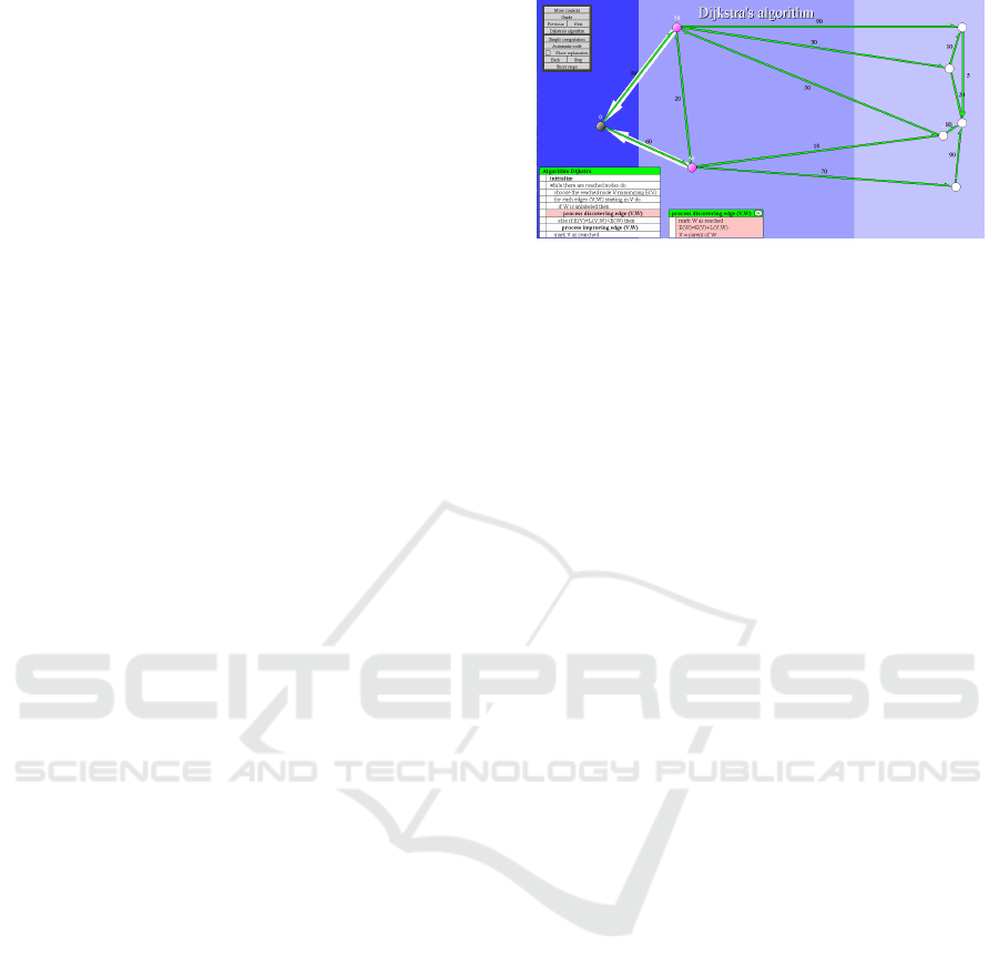
Let us note that typically a visual representation

of an invariant is not a particular visual object, but

certain organization or arrangement of the visual data.

If, e.g., each vertex v of a graph subjected to Dijk-

stra’s algorithm is labeled by a value E(v), if vertices

are classiﬁed as “processed” and “unprocessed”, and

if processed vertices are black and the unprocessed

ones are red, then the invariant

• if u is processed, and w is unprocessed, then

E(u) ≤ E(w)

can easily be visualized by moving each vertex v ho-

rizontally (i.e., keeping its y-coordinate unchanged)

to a location in which its x-coordinate is proportional

to E(v). Let us note that this also means that verti-

ces move during the computation, as their E-values

change.

In such a case there is a clearly imaginable verti-

cal line, dividing the screen to a left part containing

processed vertices, and the right one populated by un-

processed vertices. The dividing vertical line can be

explicitly drawn to make representation of the invari-

ant more explicit. Alternatively, the background color

could be different in the respective parts of the screen.

See Fig. 1 (that shows slightly more complex situa-

tion).

2 WHY VISUALIZATION USING

INVARIANTS

2.1 Algorithm Invariants

The notion of an algorithm invariant is used when pro-

ving program termination and correctness:

• Termination: Given a program P, and a statement

φ, prove that if P gets input data verifying the sta-

tement φ, the computation halts after ﬁnite num-

ber of steps.

• Partial Correctness: Given a program P, and two

statements φ and ψ, prove that if P gets input data

verifying the statement φ, and if the computation

halts after ﬁnite number of steps, the output data

verify the statement ψ.

To prove termination, it is sufﬁcient to have a

function τ and a constant c such that, given input data

verifying φ, the function τ is always non-negative and

after any c consecutive steps of the algorithm it decre-

ases by at least 1.

The standard method of solving the partial cor-

rectness problem is to ﬁnd a statement Φ such that

it implies φ at the beginning of the computation, Φ

together with the halting condition of the program P

imply ψ, and Φ remains valid throughout the whole

computation. This is why Φ is usually called an inva-

riant of the algorithm P.

Given an invariant Φ for the partial correctness

proof, proving the initial and the ﬁnal condition is

usually simple. Proving that Φ is an invariant is a

more complicated, but rather straightforward task: the

code P is split to atomic loop-less segments, and for

each segment one proves that if Φ is satisﬁed on the

entry of the segment, then it remains valid when the

segment is executed.

The main and principal problem of Program Cor-

rectness proving is to ﬁnd an invariant. The halting

problem implies that in certain cases such an invari-

ant does not exist and its existence is algorithmically

undecidable. Even if an invariant exists, it is not al-

ways clear how to ﬁnd it.

The Program Correctness theory can be used as a

theoretical background in Software Veriﬁcation, but

at least as important is a meta-theory over the Pro-

gram Correctness. It is widely accepted by many re-

searchers and teachers in Algorithm Design and Ana-

lysis that knowing an invariant of an algorithm is clo-

sely related (and some say equivalent) to understan-

ding the algorithm:

If one knows why a given algorithm always halts,

he or she usually knows some measure of “unexplored

or unprocessed data”, and such a measure can be used

as a termination counter.

Similarly, if one really understands why an al-

gorithm works correctly, he or she also knows or is

able to imagine the logical connections and relations

among the data that are processed by the algorithm.

In such a case, it is sufﬁcient to write down a descrip-

tion of all such relations in a form of a (usually rather

complex) statement Φ to get an invariant.

CSEDU 2018 - 10th International Conference on Computer Supported Education

498

On the other hand, knowledge of a termination

counter tells us (usually in a very straightforward

way) how the algorithm moves toward the end of the

computation. In some cases the function is fairy sim-

ple (e.g., the number of nodes processed by Dijkstra’s

shortest path algorithm), sometimes we have to con-

struct rather complicated “potential functions” that

measure progress of the computation, but in all cases

the way how the termination counter is constructed

gives us clear understanding why the algorithm even-

tually halts.

Similarly, an invariant is usually a generalization

of the output data condition that shows how the solu-

tion is gradually constructed.

2.2 Simple Invariant Example

A very straightforward and simple example of a ter-

mination function and an invariant can be given in the

case of Dijkstra’s shortest path algorithm. There are

many visualizations of Dijkstra’s algorithm available

in the web, e.g. (Makohon et al., 2016; DD1, ; DD2,

; DD3, ; DD4, ; DD5, ; DD6, ; DD11, ; DY1, ; DY2,

; DY3, ; DY4, ; DY5, ; DY6, ; DY7, ; DY8, ; DY9,

; DY10, ; DY11, ; DY12, ; DY13, ; DY14, ; DY15,

; DY16, ; DY17, ; DY18, ; DY19, ; DY20, ), but no

one of them tries to visualize the invariants of the al-

gorithm.

Dijkstra’s algorithm ﬁnds a shortest path from a

given vertex v

of a non-negatively edge labeled uno-

riented graph to all remaining vertices.

R ← {v

}; U ← all remaining vertices; P ←

E(v

) ← 0; E(v) ← ∞ for remaining vertices;

while R 6=

0 do

u ← the element of R minimizing E(u);

relax all edges starting in u;

move u from R to P;

end while;

Vertices of the sets U, R, P are called unreached, rea-

ched (but not yet fully processed), and processed. Re-

laxing an edge (u, v) means to perform the following

operation:

if E(v) = ∞ then move v from U to R;

E(v) = min(E(v), E(u) + L(u, v));

where L(u, v) is the length (label) of the edge (u, v).

The algorithm contains just one while loop, and

the termination is given by the following statement:

during each iteration of the loop, the (non-negative)

size of R ∪U decreases by one.

A path v

,... , v

is called deﬁnitive, if

,... , v

k−1

∈ P (v

∈ P is not required).

Figure 1: Dijkstra’s shortest path algorithm visualization.

The partial correctness is proved using the follo-

wing invariant (for details, see, e.g., (Cormen et al.,

2001)):

• for any vertex v and in any moment of computa-

tion, E(v) is the length of the shortest deﬁnitive

path from v

to v.

The correctness proof of Dijkstra’s algorithm also

uses the following auxiliary invariant:

• E(v) = ∞ if and only if v is unreached, and if v is

reached and w is processed, then E(v) ≥ E(w).

The main invariant implies immediately correct-

ness of the algorithm: at the end, all nodes accessible

from v

are processed, and hence all paths are deﬁni-

tive, and therefore E(v) is the length of the shortest

path to v.

As already mentioned above, the auxiliary invari-

ant can easily be visualized if any vertex v moves hori-

zontally during the animation so that the x-coordinate

of its location is always proportional to E(v). Such a

visualization also makes it very easy to show the va-

lidity of the main invariant, because it makes it easy

to see whether a given path is deﬁnitive. See Fig. 1,

where the domains of vertex sets P, R, U are dark,

less dark, and light, resp.

2.3 Invariant Visualization

If we accept the postulate that the algorithm under-

standing is equivalent to the knowledge of the algo-

rithm invariant, we view educational algorithm visu-

alization in a different light. The goal is not only to

visualize the data and show them changing, but we

have to arrange the data and possibly add some other

visual objects to visualize the invariant(s). Since it

often happens that relatively similar algorithms have

quite different invariants (e.g., the shortest path al-

gorithms of Dijkstra and Bellman-Ford, see the next

section), there is no general method of visualizing al-

gorithm invariants, and any such animation is unique

and incomparable with the others.

Visualization of Abstract Algorithmic Ideas

499

3 FURTHER INVARIANT

VISUALIZATION EXAMPLES

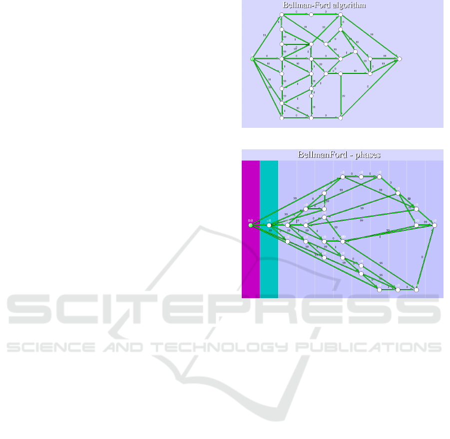
3.1 Bellman-Ford Algorithm

Bellman-Ford (BF) shortest path algorithm is very si-

milar to the method of Dijkstra mentioned in the pre-

vious subsection. It also searches for the shortest path

from a given vertex v

to all other vertices. However,

the termination proof of BF is much more difﬁcult and

completely different.

We say that a vertex v of the graph belongs to a

layer k, if k is the number of edges of the shortest

path from v

to v. (It there are more shortest paths to

v, take the minimum of such k over all shortest paths.)

Similarly as Dijkstra’s method, Bellman-Ford al-

gorithm also computes an estimation E(v) of the

length of the optimal path to v. One who knows the

BF algorithm understands that if v belongs to the layer

k, E(v) is equal to the length of the shortest path to

v for the ﬁrst time after k edge relaxations along the

path. Therefore the computation can be divided into

phases in such a way that during the k-th phase E(v)

receives the ﬁnal value exactly for vertices that belong

to the layer k.

Note that during the k-th phase, E(v) can also

change for vertices belonging to layers ` > k, but the

changed value will be changed again in later phases.

All this can easily be seen, if the way the graph

is drawn in the screen is changed as follows: starting

from the original locations of vertices, each vertex v

moves horizontally so that its x-coordinate becomes

equal to αk + β, where α and β are two positive con-

stants, and k is the index of the layer to which v be-

longs. In other ways, all vertices of the same layer

ﬁnish to belong to one vertical line, and layer indices

increase left-to-right. It is advantageous to visualize

layers better by embedding them into vertical stripe

partition of the plane, see Fig. 3.

Note also that the partition of vertices to layers is

known only after the computation is ﬁnished. There-

fore the advantageous way of visualization of the BF

computation is to run the algorithm ﬁrst in the stan-

dard way, using the initial vertex locations. Not too

much understanding is generated by the run. Then,

using the tree of the shortest paths, vertices are arran-

ged to vertical layers, and algorithm is restarted. Now,

in 20/20 hindsight, students can clearly see what has

really happened during the ﬁrst run and why it has

ﬁnished in the determined time.

Figure 2: Bellman-Ford algorithm standard visualization.

Figure 3: Bellman-Ford algorithm visualization with pha-

ses.

3.2 Binary Trees

Perhaps every one who is active in the ﬁeld of algo-

rithm animation has his or her own animation of Bi-

nary Search Tree (BST). The invariant of BST is very

easy: when vertices of the tree are scanned left-to-

right (i.e., searched in an in-order way), their labels

form a non-decreasing sequence, see Fig. 4. Howe-

ver, only few existing visualizations of BST show this

invariant. It might be argued that the BST operations

are so easy that this is not necessary (but is it neces-

sary to visualize such easy operations at all?)

It is more important to visualize advanced balan-

ced trees, like AVL-trees and red-black trees. Most

of such constructions are based on the rotation ope-

ration, see, e.g., (Cormen et al., 2001). It is very im-

portant to show that a rotation does not violate the

invariant. This can advantageously be done by ani-

mating rotation in such a way that vertices move just

vertically during rotation (see red arrows in Fig. 4),

which means that the sequence of bars representing

vertex labels does not change at all during a rotation -

a rotation preserves the invariant.

Up to our best knowledge, this simple visual trick

that clearly illustrates the principal idea of tree ba-

CSEDU 2018 - 10th International Conference on Computer Supported Education

500

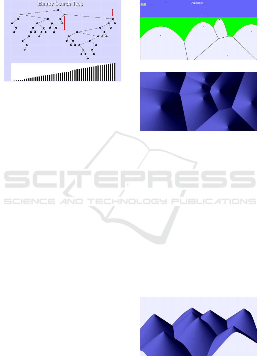
Figure 4: Binary search tree with vertex label bars.

lancing, which is the basis for all advanced tree data

structures, has never been used in connection with

tree data structure visualization.

4 ALGORITHMIC IDEA

VISUALIZATION

Even though the example given in this section can

also be understood as an algorithm invariant visua-

lization, it is perhaps more appropriate to speak about

algorithmic idea visualization (AIV). Once more,

there is no general method of AIV, because the under-

lying ideas of different algorithms in different ﬁelds

have nothing in common, and each idea is unique and

requires unique method of representation by dynamic

graphic means.

Well, in fact, there is one general method of AIV.

Even though very little is known about creative men-

tal process that leads to discovery of new algorithms,

we believe (based on our introspection) that a resear-

cher imagination is perhaps often based, as the word

suggest, on mental images - and AIV is just a straight-

forward projection of such mental images to a display

of a computer.

Due to the space restriction, we give just one ex-

ample - Fortune’s algorithm (Fortune, 1987) for Voro-

noi diagram in the plane. There are several animations

of the algorithm in the web, see (Teller, 1993; F1, ; F2,

; F3, ; F4, ; F5, ; F6, ; F7, ) - the reader is invited to

look at them. It can be seen that the Voronoi diagram

is eventually drawn, but the animations give absolu-

tely no idea what the moving arcs mean and why and

how they construct the diagram.

The algorithmic idea behind the method is fol-

lowing: imagine the plane containing sites are em-

bedded as a horizontal plane into the 3-dimensional

space. For each site, create a circular cone that has a

vertical axis and uses the site as its apex. Observe the

Figure 5: Fortune’s algorithm - planar visualization.

Figure 6: Fortune’s algorithm - cones (vertical view).

cone surfaces vertically from the inﬁnity (to avoid ef-

fects of perspective). The intersections of cones pro-

ject to the site plane as the Voronoi diagram we are

looking for. Moreover, if the “mountains” of the co-

nes are swept by an inclined plane, the intersection of

the plane with the visible parts of the cones appear as

the arcs that are visible in the planar animations (Tel-

ler, 1993; F1, ; F2, ; F3, ; F4, ; F5, ; F6, ; F7, ) and

Fig. 5. We tried to show this in Figs. 5,6,7,8,9, but the

reader is invited to look kindly to (Ku

cera, ), where he

or she can see a full visualization of the 3D situation.

5 SOFTWARE OF ALGORITHM

VISUALIZATION

A dynamic visualization system for algorithm anima-

tion should satisfy the following conditions:

• Animation speed - the system should be able to

present a good dynamic visualization.

Figure 7: Fortune’s algorithm - cones (general view).

Visualization of Abstract Algorithmic Ideas

501

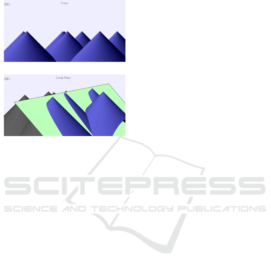
Figure 8: Fortune’s algorithm - cones (horizontal view).

Figure 9: Fortune’s algorithm - sweep plane.

• Programming effort - it should be easy to write

a visualization code.

• Widespread access - it must be easy to run a vi-

sualization code without (much of) downloading

and installing software.

Of course, the ﬁrst condition is the principal one:

in many cases, a visualization involves a continuous

transformation of the displayed picture, and it might

be computationally very demanding to deliver at least

20-25 frames per second to guarantee a smooth ani-

mation. A failure in this point would make the system

useless.

Programming languages can be divided into three

classes:

• Compiled languages - a code written by a pro-

grammer is compiled into the machine language

and runs at the maximum possible speed. Exam-

ples are the languages C and C++ that also offer

libraries of graphical functions (e.g., graphics.h).

• Semi-compiled languages - The code written by

a programmer is transformed into a simpler code

that is then interpreted by a special software. An

example is Java - the intermediate code is inter-

preted by JVM program (Java Virtual Machine)

• Interpreted languages - the runtime system re-

ads human written program instructions in run-

time and interpret them. An example is JavaS-

cript, see below.

There are really big differences in the speed

among the above classes. While one simple in-

struction is often executed in just several machine

clock tacts, if the same instruction is interpreted, the

software must ﬁrst read and parse the corresponding

code, use tables to ﬁnd the equivalent machine in-

struction, and only after that the instruction is execu-

ted. Interpreted languages are often several order of

magnitude slower than compiled languages.

Typical animations that can be found in the web

are quite simple and computationally almost trivial.

Consequently, practically any system that allows dy-

namic animation can be used, preference is given to

simple scripting languages.

However, a why visualization using algorithm

invariant visualization or any other method of vi-

sual presentation of the underlying algorithmic idea,

require sometimes computationally very demanding

processing. E.g., the visualization of Fortune’s algo-

rithm involves a 3D representation of the scene that is

composed of up to several tens of cone surfaces, each

in turn composed of several hundred of triangles (in

order to generate light effects). Moreover, user ma-

nipulation of the surface (rotation, changing between

vertical, general, and horizontal view) as well as an

animation of the plane sweep should be presented as

a smooth movie, which means that the system must

be able to deliver at least 20 frames per second. This

would suggest that at least a semi-compiled graphical

language should be used.

The bad news is that the ﬁrst condition is in a

strong conﬂict with the third condition of widespread

access: a compiled code is always speciﬁc for a par-

ticular type of processors, and a very large number of

compiled versions would be necessary to cover at le-

ast the majority of potential users. This is why the

source code is usually distributed, and a user has to

look for a compiler of the source language by himself

or herself, learn how to use it etc., which strongly li-

mits the scope of users that are able and willing to do

such installation.

The good news is that the computing power of the

recent processors is so many times higher than the real

needs of most users (perhaps with the exception of ga-

mers) that even quite slow interpreted languages are

fast enough to deliver quite good and smooth anima-

tions.

Fortunately, algorithm visualizations for teaching

purposes use small input sizes - graphs with up to se-

veral tens of nodes, matrices and vectors with few tens

of rows only, etc. which makes using interpreted lan-

guages possible.

The present paper reﬂects our experience with

an algorithm visualization system that has originally

been written in Java - a high level semi-compiled and

very powerful language. Unfortunately, Java appears

CSEDU 2018 - 10th International Conference on Computer Supported Education

502

to be too powerful in some situation and very strict

security measures are necessary if it is used as a web

application, and those security measures make using

Java much less comfortable now than it was 20 years

ago. Moreover, Java Virtual Machine must be instal-

led in a web browser or in a computer that would run

visualizations off-line, and this, even if it is a relati-

vely simple task, restricts the scope of users.

This is why we are moving the system from Java

to JavaScript using the fact that the latter language

is essentially ubiquitous - it is difﬁcult to imagine a

personal computer without a web browser (Chrome,

Mozilla, Explorer, Opera, etc.), and all standard web

browser come with a JavaScript interpreter (which is

enabled by default). A user does not need to do more

than to ﬁnd the proper web page and perform 3 ob-

vious clicks to open a selected visualization of our

collection. In this way, our system is going to be avai-

lable to literally any user of the web and requires no

installation of any software (assuming that a browser

is available).

At the present time we have moved the most com-

putationally difﬁcult item of our collection - visua-

lization of Fortune’s algorithm for ﬁnding a Voronoi

diagram in the plane - from Java to JavaScript. The

visualization of Fortune involves a very complex 3D

visualization of a surface composed of a number of

cones under light coming from the left. It is substan-

tially more difﬁcult that other 3D visualization of our

collection. The application allows a user to rotate the

surface in two directions and animate sweeping the

surface by an inclined plane, and we have found that

a JavaScript code is executed sufﬁciently fast even

on smart-phones and tablets (which, fortunately, have

smaller displays, which limits the size and complexity

of the displayed scene).

The reviewer is kindly invited to play with the vi-

sualization of Fortune algorithm at the URL (Ku

cera,

) to see that the speed of simulation might be limi-

ting if the number of sites is too high, but it is quite

sufﬁcient for the standard educational use.

Thus, the ﬁrst condition has a threshold nature - if

the hardware is fast enough to compensate the inter-

preter slow-down for inputs of sizes typical for educa-

tional purposes, it is possible to forget it and concen-

trate on the third condition that can be fully satisﬁed

by a graphical script language that is embedded into

all standard web browsers.

There is still the second condition - how much pro-

grammer’s time and effort is needed. The second con-

dition is also in contradiction to the last one - simple

interpreted script languages are designed for writing

simple applications, but good algorithm visualization

with educational value could be quite complex soft-

ware products of thousands code lines. It would be

much more convenient to write such large codes in

an object-oriented language with a strict type control

(like Java and C++) that is supported by advanced de-

velopment tools (like Eclipse and Net Beans). There

are also extensions of script languages that bring at

least a part of the comfort of more advances systems.

However, we have found another tool that makes

writing JavaScript algorithm visualizations relatively

easy and fast - a strong programmer’s discipline. An

experienced programmer that is able to write natural

and easy readable programs, does not need to be ob-

served and directed by a development environment,

and avoids seductions of ‘easy’ tricks of script langua-

ges, is not much less productive in JavaScript than,

e.g., in Java. A beneﬁt is a code that can be run by

essentially each web user without any system instal-

lations.

REFERENCES

Algoanim. algoanim.ide.sk.

AlgoLiang. cs.armstrong.edu/liang/animation/animation.html.

Algomation. www.algomation.com.

Algoviz. www.algoviz.org/biblio/authors; (a super-

reference: a web page containing several hundreds

of references to algorithm visualizations and anima-

tions).

bassat Levy, R. B. and Ben-Ari, M. (2007). We work so hard

and they don’t use it: acceptance of software tools by

teachers. In ITiCSE ’07: Proceedings of the 12th an-

nual SIGCSE conference on Innovation and techno-

logy in computer science education, Dundee, Scot-

land. ACM Press.

Brown, M. and Sedgewick, R. (1985). Techniques for algo-

rithm animation. IEEE Software, 2:28–39.

Brown, M. H. (1988). Algorithm Animation. MIT Press.

Cormen, T. H., Leiserson, C. E., Rivest, R. L., and Stein, C.

(2001). Introduction to Algorithms, 2nd edition. The

MIT Press, Cambridge, Massachusetts, and McGraw

Hill, Boston.

DD1. A demo in en.wikipedia.org/wiki/dijkstra’s algorithm.

DD11. jhave.org/algorithms/graphs/dijkstra/dijkstra.shtml.

DD2. www.cs.usfca.edu/ galles/visualization/dijkstra.html.

DD3. people.ok.ubc.ca/ylucet/ds/dijkstra.html.

DD4. www-m9.ma.tum.de/graph-algorithms/spp-

dijkstra/index en.html.

DD5. qiao.github.io/pathﬁnding.js/visual/.

DD6. pckujawa.github.io/portfolio/net-dijkstra/.

DY1. www.youtube.com/watch?v=pvfj6mxhdmw.

DY10. www.youtube.com/watch?v=kvrwplnioem.

DY11. www.youtube.com/watch?v=cl1bylngb5q.

DY12. www.youtube.com/watch?v= lhsawdgxpi.

DY13. www.youtube.com/watch?v=wt5cqvfdyxg.

DY14. www.youtube.com/watch?v=0nvyi3o161a.

Visualization of Abstract Algorithmic Ideas

503

DY15. www.youtube.com/watch?v=lfb8qkxzhy0.

DY16. www.youtube.com/watch?v=1057z9xtfcs.

DY17. www.youtube.com/watch?v=ug7vmpwkjma.

DY18. www.youtube.com/watch?v=kowij71jdc4.

DY19. www.youtube.com/watch?v=cbow7y2udq8.

DY2. www.youtube.com/watch?v=gdmfowyqlci.

DY20. www.youtube.com/watch?v=mv4r7f82doa.

DY3. www.youtube.com/watch?v=wn3rb9wvydy.

DY4. www.youtube.com/watch?v=5gt5hyzjnoo.

DY5. www.youtube.com/watch?v=jwemgqncz8q.

DY6. www.youtube.com/watch?v=8ls1rqhcopw.

DY7. www.youtube.com/watch?v=p4ukmd1tfri.

DY8. www.youtube.com/watch?v=laxzgercdf4.

DY9. www.youtube.com/watch?v=4xrotuo1xaw.

F1. www.raymondhill.net/voronoi/rhill-voronoi.html.

F2. tech.io/playgrounds/243/voronoi-diagram/fortunes-

algorithm.

F3. www.diku.dk/hjemmesider/studerende/duff/fortune.

F4. philogb.github.io/blog/2010/02/12/voronoi-tessellation.

F5. www.youtube.com/watch?v=k2p9ywsmaxe.

F6. www.youtube.com/watch?v=kuqriq3mzcy.

F7. www.youtube.com/watch?v=pcaxgsc-gx.

Fortune, S. (1987). A sweepline algorithm for voronoi dia-

grams. Algorithmica, 2:153–174.

cera, L. www.algovision.org.

Makohon, I., Nguyen, D. T., Sosonkina, M., Shen, Y., and

Ng, M. (2016). Java based visualization and anima-

tion for teaching the dijkstra shortest path algorithm

in transportation networks. Int. J. Software Eng. &

Appl., 7(3):11–25.

Teller, S. J. (1993). Visualizing fortune’s sweepline algo-

rithm for planar voronoi diagrams. In Symposium on

Computational Geometry, San Diego, page 393.

VisuAlgo. visualgo.net.

CSEDU 2018 - 10th International Conference on Computer Supported Education

504