Reconstruction of Piecewise-explicit Surfaces from
Three-dimensional Polylines
Applications in Seismic Interpretation in Compressive Domain
Joseph Baudrillard
1,2
, S
´
ebastien Guillon
2
, Jean-Marc Chassery
1
, Mich
`
ele Rombaut
1
and Kai Wang
1
1
GIPSA-Lab, 11 rue des math
´
ematiques, Grenoble Campus BP46, F-38402 Saint-Martin d’H
`
eres, France
2
TOTAL SA, CSTJF, Avenue Larribau, 64000 Pau, France
{jean-marc.chassery, michele.rombaut, kai.wang}@gipsa-lab.grenoble-inp.fr
1 RESEARCH PROBLEM
Oil and gas exploration relies heavily on the knowl-
edge of the underground structure. By conducting
seismic reflection surveys, an image of the subsurface
is obtained in the form of a 3D “cube”, on which geo-
logical objects are interpreted. Amongst them, depo-
sition surfaces (called horizons) are numerically mod-
eled in order to assess the economical potential of a
hydrocarbon field.
The use of geo-referenced heightmaps is standard
practice to represent horizons as they are mostly hor-
izontal surfaces. In our context a heightmap is a ge-
olocalized image, whose pixel values are a vertical
elevation distance. However horizons are not always
explicit; in other words, they cannot be projected ver-
tically on a heightmap anymore. Yet many geological
structures lead to the interpretation of such horizons,
for example inverse faults in compressive domain.
They are called “multivalued” as several height values
are associated to the surface at some locations on the
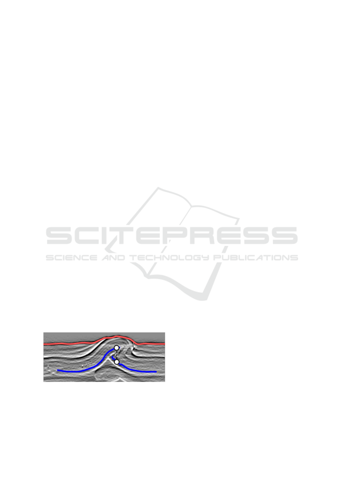
heightmap (see figure 1). For practical reasons, hori-
zons are typically defined by hand-picked polylines.
They are then vertically projected on a heightmap as
pixels that are interpolated in a process called “grid-
ding”, in order to create a dense continuous surface.
Figure 1: Monovalued (top) and multivalued (bottom) hori-
zons interpreted on a seismic section. At some heightmap
location (corresponding to a vertical dashed line in this sec-
tion view), 2 points are required to describe the multivalued
(bottom) surface.
A new model is therefore required in order to
represent a multivalued horizon, as well as methods
to reconstruct it by interpolation from sparse three
dimensional polylines. We propose here to use a
piecewise-explicit representation called a patch sys-
tem, i.e. a set of heightmaps that can be topologi-
cally connected at the pixel level. This new model is a
natural extension of the heightmap, scales seamlessly
from standard monovalued horizons to complex mul-
tivalued surfaces, is memory efficient and almost as
fast as a simple heightmap. Moreover, we will show
how monovalued interpolation methods can be easily
adapted to this new model.
2 OUTLINE OF OBJECTIVES
Our objective is to provide tools to handle multivalued
horizons in the structural interpretation process. The
following problems must hence be adressed:
• Extend the heightmap model for multivalued hori-
zons in order to have a digital representation of the
geological objects it is associated with
• Develop a surface reconstruction process so that
the new model can be created by interpolation of
a set of sparse polylines
3 STATE OF THE ART
Geographic Information Systems (GIS) typically con-
struct elevation models in the form of heightmaps
that are interpolated using gridding methods (Briggs,
1974; Smith and Wessel, 1990). A heightmap is an
example of explicit representation, and hence cannot
represent multivalued horizons. There are however
other numerical models able to represent a multival-
8
Baudrillard, J., Guillon, S., Chassery, J., Rombaut, M. and Wang, K.
Reconstruction of Piecewise-explicit Surfaces from Three-dimensional Polylines.
In Doctoral Consortium (GISTAM 2018), pages 8-18
Copyright
c
2019 by SCITEPRESS – Science and Technology Publications, Lda. All rights reserved
ued horizon which can be built by from sparse geo-
logical data.
Point clouds can indeed be used (Levoy and
Whitted, 1985). Triangulated surfaces (meshes) can
be constructed from seismic data (Sadri and Singh,
2014). Various approaches also exist to interpolate
closed meshes from contours but they cannot cope
with open surfaces (Zou et al., 2015). Alternatively,
one could consider using voxels to represent a surface,
though this requires using memory efficient spatial in-
dex structures such as voxel octrees (Meagher, 1982)
or R-tree variants (Beckmann et al., 1990). A surface
can also be parameterized into an image (Hormann
et al., 2007), but knowledge of the complete surface
is needed, which is not our case as we interpolate it
from polylines.
In the next section, we will show that these al-
ternative models perform significantly worse than a
heightmap when it comes to representing horizons,
and prevent a unified representation of monovalued
horizons with heightmaps and multivalued horizons.
Instead, a new model extending the heightmap to
piecewise-explicit surfaces will be used. This new
model will also support gridding without major mod-
ification.
4 METHODOLOGY
4.1 A New Horizon Model: The Patch
System
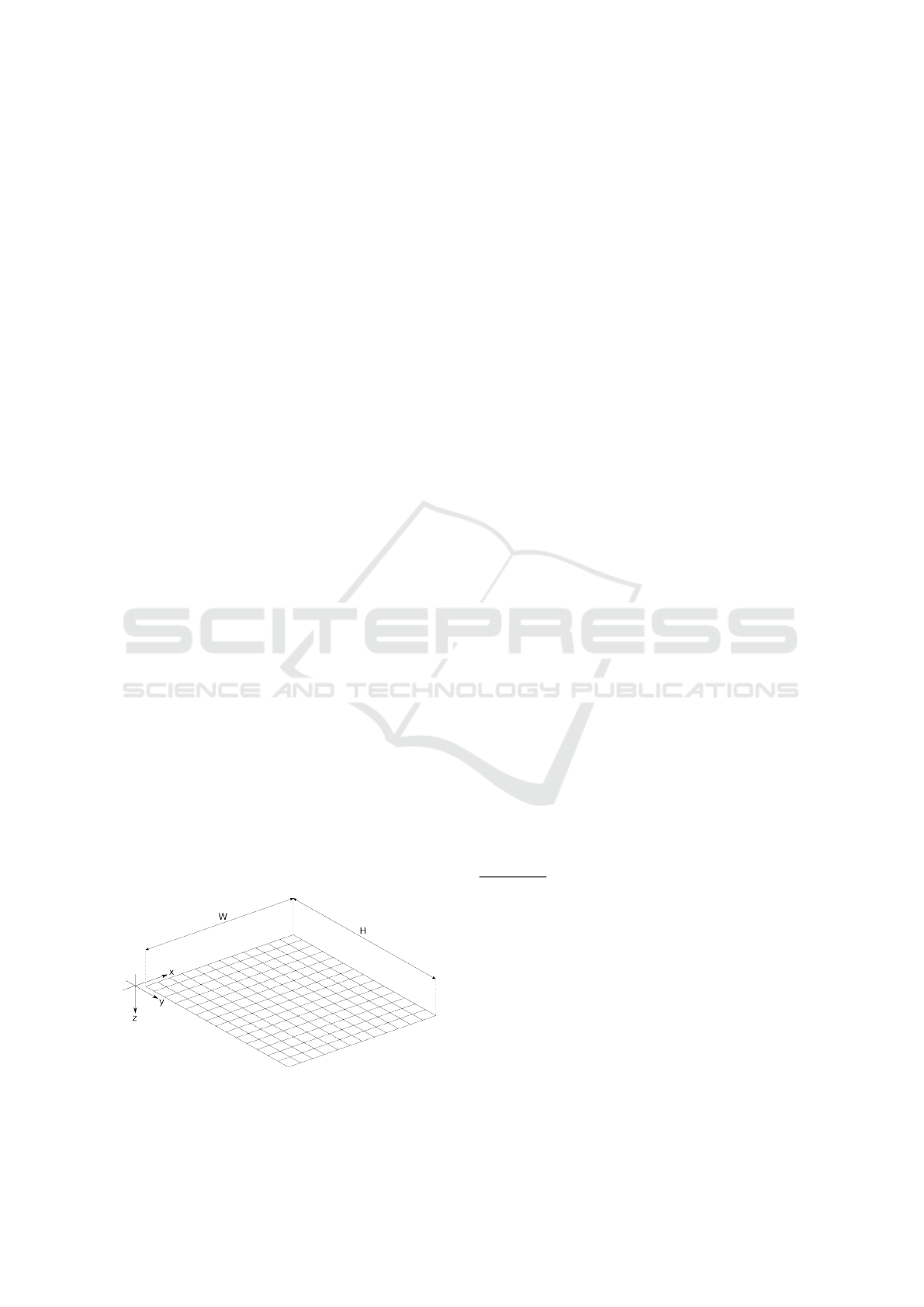
The whole problem takes place in a seismic survey
of horizontal dimensions W × H pixels, the horizon-
tal plane being associated to the first two coordinates
(x, y) of a 3D point (x, y, z). It is illustrated in figure 2.
Noting Ja, bK the set {n ∈ N, a ≤ n, n ≤ b}, we there-
fore define the survey domain D such as:
D = J0,W − 1K × J0, H − 1K (1)
Figure 2: The survey 2D grid within 3D space.
4.1.1 Motivations and Orders of Magnitude
For explicit (monovalued) horizons, the heightmap is
a really efficient model: pixels can be accessed in con-
stant time because of their implicit location, and an
image is also a very compact data structure in mem-
ory. It can easily be displayed as a map, or triangu-
lated into a mesh. In other words it has a simple data
model, and can be quickly created, displayed or pro-
cessed.
Seismic surveys can reach large dimensions (hun-
dreds of gigabytes on disk). A heightmap on this
kind of survey can therefore be an image dozens of
megapixels large, and many are routinely computed
during a study. Moreover, many geophysical pro-
cesses and methods were developed as image process-
ing algorithms and hence require the regular sampling
of a heightmap. Using a radically different model
such as a mesh would lead to significant methodol-
ogy change and software refactoring.
We complemented these qualitative arguments by
a benchmark. It compared the performance of all
models mentioned in section 3 in typical usage sit-
uations (IO, display, storage). The quantitative results
we gathered confirmed our initial project to keep us-
ing an explicit representation (the heightmap) as the
model for multivalued horizons. It must however be
changed in order to cope with vertically superposed
horizon parts that come with multivalued surfaces.
4.1.2 Model Proposal
The proposed extension of heightmaps to multivalued
horizons is a set of connected heightmaps, called a
patch system. The idea is to use as many heightmaps
as required: two vertically superposed points must
indeed belong to two separate heightmaps. We also
want to support connections between pixels of differ-
ent heightmaps so a complete connected surface can
be described (see figure 3).
Definition: More formally, a patch system P made of
N
P
patches P
i
can be defined as:
P = {P
i
, i ∈ J0,N
P
− 1K} (2)
Each patch P
i
is defined as:
P
i
= {H
i
, N
i
} (3)
Where:
• H
i
is the patch heightmap, storing the geometry of
the patch:
H
i
:
(
D → R
(x, y) 7→ Patch height z at (x, y)
(4)
Reconstruction of Piecewise-explicit Surfaces from Three-dimensional Polylines
9
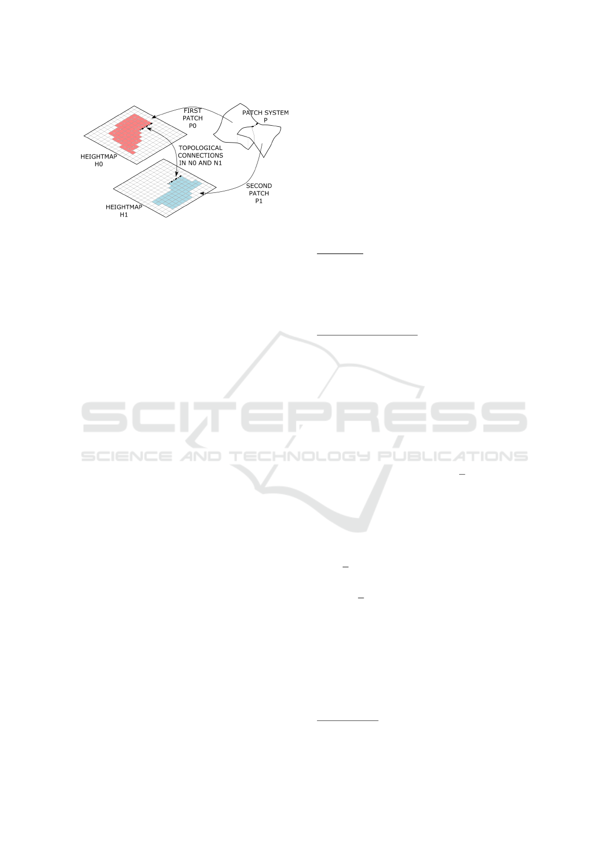
Figure 3: An example of multivalued surface described by a
patch system made of two patches P
0
and P
1
. The geometry
is stored in the two heightmaps H
0
and H
1
, whereas the per-
pixel topological connections between the two patches are
stored in the two neighbor data structure N
0
and N
1
.
• N
i
is the so-called neighbor data structure con-
taining the neighborhood information. Namely it
provides the natural pixel neighbors of any pixel
of heightmap H
i
, and if necessary the pixel neigh-
bors in another patch P
j
, j 6= i. The latter only oc-
curs for pixels touching another patch, i.e. on the
“edges” of a patch. This structure stores the topol-
ogy of the patch system, and can typically be con-
structed as a neighbor patch index map that pro-
vides for each pixel a list of neighbors. A neigh-
bor in this list is a pair of patch index and neighbor
index (for example, from 0 to 3 for the four Von
Neumann neighbors). This is made space efficient
by omitting neighbors that are in the same patch,
in other words neighbors with the same patch in-
dex.
It follows that a patch system is a piecewise-
explicit representation of a multivalued horizon, and
benefits from the efficiency of the heightmap model
for both storage and access. Our model elegantly ex-
tends the heightmap, and a monovalued horizon can
be seen as a patch system with a single patch, without
any useless overhead or complexity being introduced.
We will demonstrate how standard interpolation al-
gorithms can be adapted to this model in section 4.2,
given a properly defined patch system. The construc-
tion of such a well-formed patch system from sparse
polylines is the subject of sections 4.3 and 4.4.
4.2 Horizon Interpolation: The
Gridding Process
We will present here a standard horizon interpolation
method, and how it can be naturally adapted to a mul-
tivalued horizon represented by a patch system.
4.2.1 Monovalued Case
Monovalued horizons are represented by heightmaps.
For practical reasons heightmaps are constructed by
interpolation of a set of sparse polylines, picked by
geologists on the seismic cube. In this context the
interpolation process is called gridding. Many in-
terpolation methods can be used (inverse-distance
weighting, kriging) but we chose a variational ap-
proach (Briggs, 1974; Smith and Wessel, 1990) which
is straightforward, efficient and robust towards con-
straint density anisotropy.
Objectives: Given a set of constraint height values f
i, j
to respect at positions (i, j), the objective is to find the
unknown heights elsewhere on the heightmap, while
creating a smooth surface. This can be formulated
as the search for an unknown function f : D 7→ R
that takes the values f
i, j
at locations (i, j) while be-
ing smooth.
Variational Formulation: Let Ω be the set of locations
where the height is known. Horizon gridding can be
seen as a minimization problem of a quantity J( f )
defined by two components D( f ) and L( f ), the first
quantifying how close the surface is to the constraint
heights, the second measuring the “smoothness” of
the final surface:
J( f ) = D( f ) + L( f ) (5)
Where:
• D( f ) is the constraint term that imposes f to pass
through known values at locations in Ω. It is de-
fined as:
D( f ) = || f · δ − f ||
2
(6)
With:
– δ being the selection function such as:
δ :
D → {0, 1}
(i, j) 7→
(
1 if (i, j) ∈ Ω
2
0 otherwise
(7)
– f is f evaluated at locations in Ω:
f :
D → R
(i, j) 7→
(
f
i, j
if (i, j) ∈ Ω
2
0 otherwise
(8)
• L( f ) is the smoothness term. In our case we
want to minimize the variations and curvature of f
which is expressed using a linear combination of
the gradient and Laplace operators, as they pro-
vide an image of the local slope and curvature re-
spectively
1
:
L( f ) = α||∇ f ||
2
+ β||∆ f ||
2
(9)
1
As written, L( f ) prevents an exact passage through
constraints but this is acceptable in our context
DCGISTAM 2018 - Doctoral Consortium on Geographical Information Systems Theory, Applications and Management
10
The Gridding Equation: We want to minimize the
quantity J( f ) = || f · δ − f ||
2
+ α||∇ f ||
2
+ β||∆ f ||
2
.
This is reached when
∂J
∂ f
= 0, which leads to:
(α∆ + β∆
2
+ δ) f = f (10)
The parameters α and β in equations 9 and 10 can
be made small in order to have a surface closer to in-
put constraints. Conversely, big values lead to a very
smooth surface that might respect constraints more
loosely. Control over uncertainties can therefore be
obtained using relevant parameter values.
Numerical Implementation: When evaluated numer-
ically using the finite difference method, by noting
n = W ·H and by mapping the survey grid on a vector
of R
n
, it can be shown that this leads to the definition
of a matrix equation in the form:
A · X = B (11)
where:
• A is an n × n matrix representing the action of op-
erator (α∆ + β∆
2
+ δ), i.e. the access to neighbor
pixels
• X is a vector of R
n
containing the unknown height
pixels f
• B is a vector of R
n
containing 0 for pixels without
constraints, and the known height f for constraint
pixels
Monovalued gridding is performed by first raster-
izing the polylines onto the heightmap, using standard
algorithms (Bresenham, 1965). Pixel positions and
heights are interpolated between polyline vertices in
this process. Equation 11 can then be solved by a
direct or iterative method (Jacobi, Gauss-Seidel, con-
jugate gradient, etc.). Implementations are presented
in details in the literature (Walter, 2014).
Figure 4 illustrates the gridding of some projected
polylines on a heightmap. Note that not all pixels of
the heightmap become valued (the surface does not
takes all the image). Indeed, gridding only takes place
in what we call the envelope of the horizon, i.e. the
pixel locations where it should be defined. Outside
envelope, extrapolation would occur instead of inter-
polation
2
.
4.2.2 Multivalued Case
When looking at equation 11, we see that only the
connectivity information stored in A depends on the
horizon type: it is a simple access to natural pixel
2
The actual definition of an envelope for monovalued
horizons and how it prevents pixels from being gridded are
not detailed here for the sake of brevity
Figure 4: An example of monovalued gridding. Sparse con-
straint pixels from rasterized polylines (left) are interpolated
into a dense surface (right).
neighbors in the case of a monovalued horizon, and
becomes slightly more complex in the case of a mul-
tivalued horizon – a patch pixel can have neighbors in
another patch. In order to grid multivalued horizons,
we define an extended unknown vector X
E
that con-
tains the unknown heights X
i
associated to all patches
P
i
simultaneously:
X
E
=
X
1
.
.
.
X
N
(12)
Using the connectivity information given by the
neighbor data structure presented in section 4.1.2, it
is possible to construct the extended operator matrix
A
E
and the extended constraint vector B
E
in a similar
manner and therefore interpolate each patch correctly.
Equation 11 then becomes:
A
E
· X
E
= B
E
(13)
Interpolation of a multivalued horizon in the form
of a patch system is then a natural extension of mono-
valued gridding. However, given just a set of input
polylines, in order to prepare a patch system for grid-
ding, we must first provide a solution to a partitioning
problem (section 4.3) and an envelope computation
problem (section 4.4).
4.3 Partitioning Problem
Geologists interpret polylines in vertical slices of the
cube called sections. Each input polyline is therefore
constrained into a vertical plane, that can be shared
between several polylines (see figure 5). Polylines are
also intersecting each others geometrically but do not
share any vertex.
Vertices are therefore introduced in order to have
polylines intersect at the exact location of a vertex.
At this point the set of polylines can be seen as a con-
nected graph named G. The objective is now to find
a decomposition into a set of monovalued sub-graphs
G
i
, i.e. sub-graphs where no vertical overlap occurs.
Reconstruction of Piecewise-explicit Surfaces from Three-dimensional Polylines
11
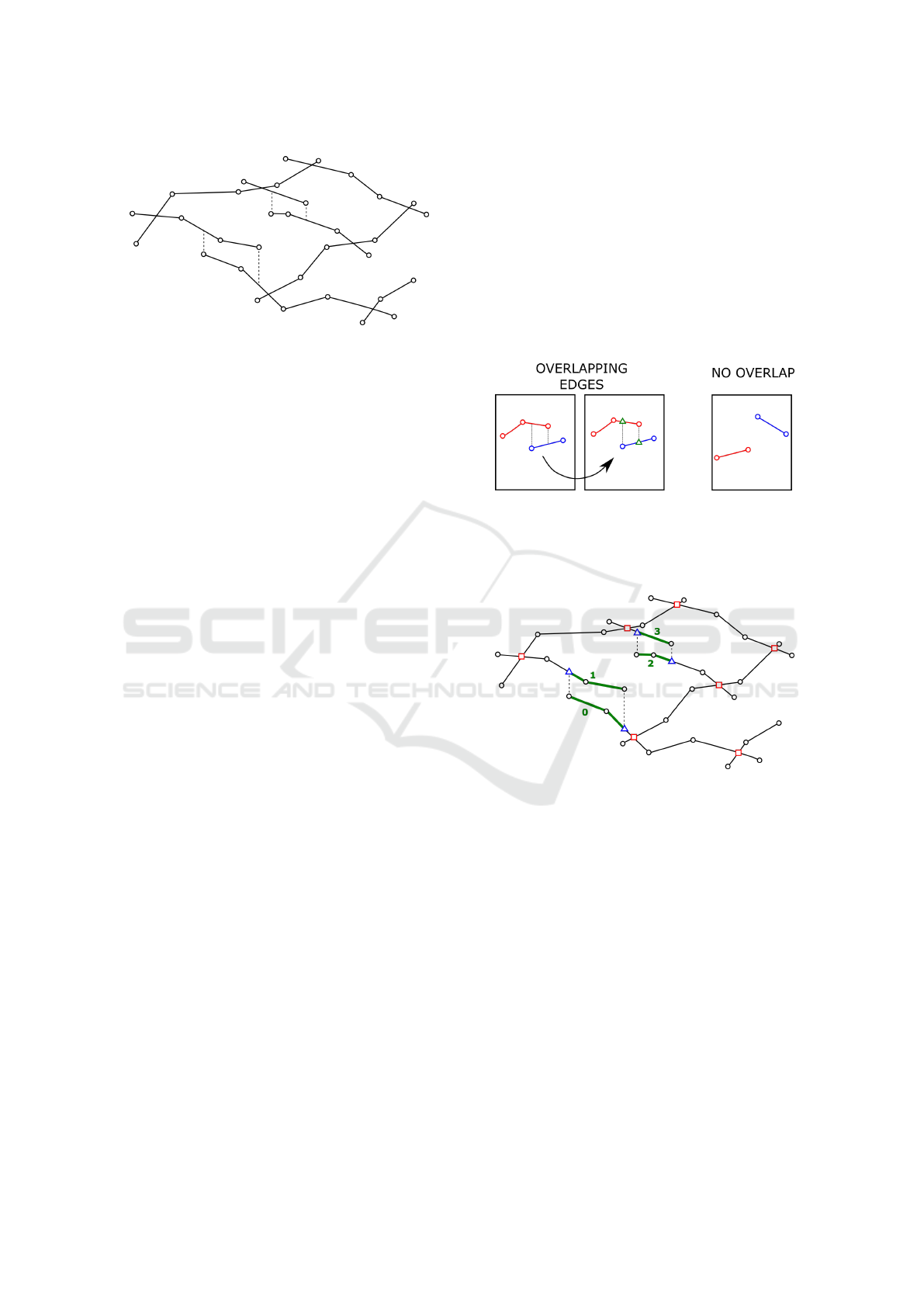
Figure 5: An example of input polylines. Note they are
intersecting but not necessary at the location of a polyline
vertex. Some polylines are co-planar and display partial
edge superpositions, depicted with dashed lines.
Such decomposition is not unique, therefore some cri-
teria must be defined in order to choose a suitable par-
tition.
After a partition is found, each sub-graph will be
turned into a patch heightmap in the envelope com-
putation stage, and will then be gridded. Both these
steps have a computational complexity of O(N ·W ·H)
where N is the number of patch in the patch system,
W and H are the width and height of the patch. This
means we want to reduce the number of patch (so the
number of sub-graphs G
i
) as much as possible, and
large patch size must be avoided – this is a second or-
der concern though as only the envelope will be con-
sidered, not the entire heightmap image.
Considering the partitioning problem in a varia-
tional framework could provide an optimal combina-
tion of patch count and size, but would be prohibitive
to evaluate, graph partitioning problems often being
NP-hard (Buluc et al., 2013). In this context, we pro-
pose instead a constructive method that leads to an
acceptable compromise between patch count and size.
The approach is based on three steps:
• Multivalued Scan. Vertically superposed edges
of G are detected, grouped into superposed zones,
and vertices are introduced in order to avoid hav-
ing half-superposed edges (see section 4.3.1)
• Sub-graph Index Propagation. Simultaneous
propagation of sub-graph index from superposed
zones leads to the definition of monovalued sub-
graphs G
i
(see section 4.3.2)
• Merge. Reduce sub-graph count by merging to-
gether those that can be. The sub-graphs after
merge are noted
˜
G
i
(see section 4.3.3)
4.3.1 Multivalued Scan
As previoulsy said, polylines belong to vertical
planes. This means polylines in the same plane can
be vertically superposed. There is no reason for two
edges to be entirely superposed though, and in order
to simplify the following processes we introduce a
vertex whenever necessary so that an edge is either
completely superposed with another, or is not at all
(see figure 6). Once these vertices are introduced, de-
tecting vertically superposed edges is a simple geo-
metric problem. Superposed edges are then grouped
by connected components named superposed zones.
These zones are given a unique index that will be
used in the sub-graph index propagation. The result-
ing graph is illustrated by figure 7.
Figure 6: Two polylines picked in the same section are
either superposed (left) or not (right). When they are su-
perposed, vertices (symbolized here by triangles) are intro-
duced in order to only have edges that are totally overlap-
ping, or not at all.
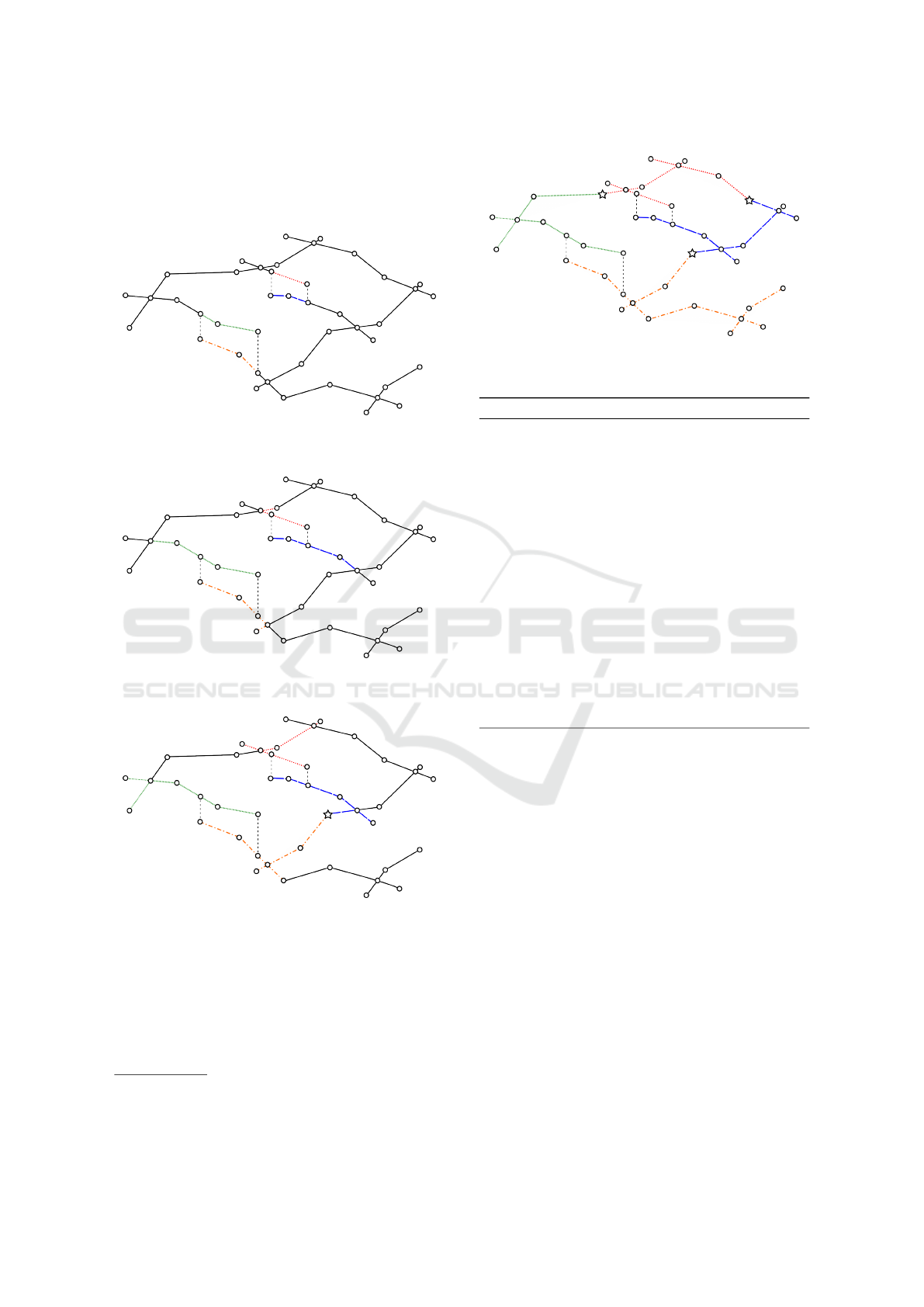
Figure 7: The input polylines after multivalued scan. Red
(square) vertices were introduced in order to have polylines
intersect precisely at a vertex location. Blue (triangle) ver-
tices were added in order to simplify the superposed sta-
tus of an edge. Superposed edges detected in the multival-
ued scan are reported in green (thick), and grouped by con-
nected component named superposed zones that are given a
unique index (here from 0 to 3).
4.3.2 Sub-graph Index Propagation
At this point, for each superposed zone given the in-
dex i, we initialize a monovalued sub-graph G
i
with
the superposed zone’s edges. The sub-graphs G
i
are
called monovalued as by construction, each is made
of edges that do not overlap. All the graph edges
can then be indexed using a propagation method il-
lustrated by algorithm 1.
This ensures that all edges will have a sub-graph
index, but more importantly that each index will be
DCGISTAM 2018 - Doctoral Consortium on Geographical Information Systems Theory, Applications and Management
12
associated with a similar number of edges
3
. Follow-
ing the previous example, figures 8, 9, 10 and 11 are
showing the evolution of the sub-graph index propa-
gation in the graph.
Figure 8: Before propagation, only superposed zones are
given an index, symbolized here by a color and a line style.
Figure 9: After 2 steps, sub-graphs are starting to extend.
Using a FIFO list balances their size (see algorithm 1).
Figure 10: After 6 steps, some superposed zones have met
each other at a vertex indicated by a star. Propagation will
continue on other fronts as all edges are not indexed yet.
3
Exact same number is not reached as it depends on the
graph shape for propagation. In practice sub-graphs have
edge counts on the same order of magnitude though
Figure 11: End of propagation: every edge has a sub-graph
index.
Algorithm 1 : Sub-graph index propagation.
Procedure propagate (G, {G
i
})
Input:
G . Connected input graph
{G
i
} . Indexed sub-graphs (superposed
zones only at start)
Algorithm:
1: edges ← FIFO list with all edges of {G
i
}
2: while edges is not empty do
3: Pop a, the first edge of edges
4: for Each unindexed edge b touching a do
5: index ← a’s index
6: Index b with index
7: Add b to edges
8: end for
9: Add a to G
index
10: end while
End procedure
4.3.3 Merge
By starting from superposed zones, sub-graph index
propagation ensures that enough monovalued sub-
graphs will be used. However it can lead to a massive
over-estimation of the number of required sub-graphs,
especially when the picking is dense. This being said,
it occurs that many of the sub-graphs can be merged
together: namely such merge is possible if they do not
overlap vertically.
Merging is hence performed by considering each
pair of sub-graphs (G
i
, G
j
), i 6= j. If they are con-
nected by a vertex and do not overlap vertically, they
are merged together. An example of merging can be
found in figure 12. We call
˜
G
i
the merged sub-graphs.
4.4 Envelope Computation
At this point the partitioning problem is solved as we
found a partition of G into a relatively low number of
monovalued sub-graphs
˜
G
i
. In order for a sub-graph
Reconstruction of Piecewise-explicit Surfaces from Three-dimensional Polylines
13
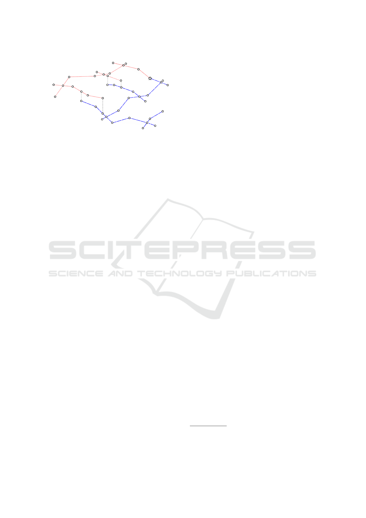
Figure 12: After considering each pair of connected sub-
graphs for merging, only two big sub-graphs remain (red-
points and blue-dashed). Also notice there is now only one
junction vertex (star) anymore.
˜
G
i
to be gridded, it is however necessary to convert it
to a patch P
i
and compute its envelope. As detailed in
the next section, each sub-graph will indeed be con-
verted into a heightmap, and its polylines will be ras-
terized into constraint pixels.
For a patch P
i
, the envelope is the combination of
two objects:
• A mask indicating for each pixel of its heightmap
H
i
whether it is to be gridded or not. This
mask will be encoded in the heightmap H
i
using
a boolean value, for example true if inside en-
velopes, f alse otherwise
• A set of junction points, i.e. pixels that have
neighbor pixels in another patch. This will be en-
coded in the neighbor data structure N
i
The envelope will therefore be the domain around
constraint pixels, i.e. pixels coming from poly-
lines. There are methods to compute the envelope (or
“hull”) of a set of pixels: one could consider using the
pixels’ convex shape (Kirkpatrick and Seidel, 1986)
or alpha shape (Edelsbrunner et al., 1983), but in our
case this lead to masks that are too large and hence
does not prevent extrapolation.
An efficient and intuitive way to construct this
mask is instead to use the closing morphological op-
erator against the constraint pixels of each heightmap.
Closing is actually the succession of a dilatation and
an erosion, both using a structural element of size d
C
pixels. When a relevant value of d
C
is chosen, holes
between polylines are closed by the dilatation while
extrapolation is avoided because of the erosion. We
therefore propose the following steps to find the en-
velope of each patch:
• Heigtmap Conversion. Turn each sub-graph
˜
G
i
into a patch heightmap H
i
initialized with con-
straint pixels (see section 4.4.1)
• Dilatation. A dilated envelope is created indepen-
dently for each patch (see section 4.4.2)
• Dilated Envelope Restriction and Junction
Point Location. For each patch pair that is con-
nected topologically by a vertex of G, restrict
dilated envelopes to ensure smooth connection
along a set of junction points (see section 4.4.3)
• Joint Erosion. Each dilated envelope is eroded
to prevent extrapolation. This is done simultane-
ously, i.e. on the multivalued surface (see section
4.4.4)
4.4.1 Heightmap Conversion
After a partition is found, each sub-graph can be con-
verted to an image of size W ×H, the survey size (see
figure 13). We therefore associate each sub-graph
˜
G
i
with its corresponding patch P
i
of heightmap H
i
whose pixel (x, y) contains the height z for any vertex
(x, y, z) in
˜
G
i
:
H
i
:
D → R
(x, y) 7→
z
0
if ∃M
0
= (x
0
, y
0
, z
0
) ∈
˜
G
i
,
(x, y) = (x
0
, y
0
)
ν (null value) otherwise
(14)
Remarks:
• ν (null value) is a magic value designating a patch
pixel that is not yet valued (it is not a constraint
pixel). The value of such a pixel will be set during
gridding
• Between graph vertices, edges are rasterized on
the heightmap and the end vertices’ heights inter-
polated
• The “intra-patch” connectivity information once
stored explicitly in the edges of
˜
G
i
is now replaced
by the natural neighborhood of the pixels in P
i
.
The “inter-patch” connectivity, i.e. the topologi-
cal connection between
˜
G
i
and its potential neigh-
bor sub-graphs is for now lost though, but it will
be stored in the neighbor data structure N
i
in sec-
tions 4.4.3 and 4.4.4
4.4.2 Dilatation
Although image morphological operators are typi-
cally defined by kernels associated with structural ele-
ments, numerical implementations are faster when us-
ing Euclidean Distance Maps (EDM). It can be shown
that both dilatation and erosion are equivalent to the
thresholding of an EDM
4
(Russ, 1998). Using an
4
This is for disk-shaped structural elements and distance
maps based on the L2 norm, because the disk is the topolog-
ical ball associated with the L2 norm in R
2
DCGISTAM 2018 - Doctoral Consortium on Geographical Information Systems Theory, Applications and Management
14
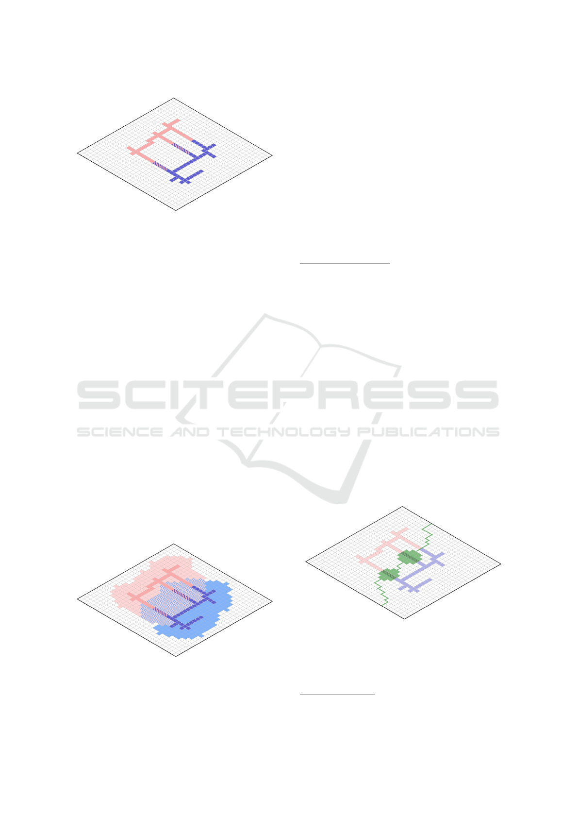
Figure 13: Following the example in figure 12, each sub-
graph G
i
is converted into a heightmap H
i
. The superposed
result is displayed here. Overlapping edges in G lead to
overlapping pixels in this image (pixels with stripes).
EDM is faster than using masks because there are effi-
cient O(W · H) algorithms to compute a distance map
(Danielsson, 1980; Treister and Haber, 2016). These
algorithms typically introduce numerical errors, but
they are tolerable in our case as the envelope does
not require pixel-perfect precision and those errors are
small (Grevera, 2004).
Recall constraints are the non-ν pixels of
heightmap H
i
. We therefore construct the map of
distance to constraints DC
i
. Being a distance map,
each pixel of DC
i
has a positive value and is only zero
on the location of constraints, i.e. ν pixels. DC
i
is
defined by:
DC
i
:
(
D → R
+
(x, y) 7→ distance to closest non-ν pixel
(15)
We then define the dilated envelope DE
i
by
thresholding the distance map DC
i
:
DE
i
= {(x, y) ∈ D, DC
i
(x, y) ≤ d
C
} (16)
Using this thresholding method, it is possible to
obtain the dilated envelopes, as depicted by figure 14.
Figure 14: An example of dilated envelopes. They overlap
when constraints of the two patches are both closer than d
C
(overlapping dilated envelopes correspond to checkerboard
pixels).
4.4.3 Dilated Envelope Restriction and Junction
Point Location
Before computing the erosion, we want dilated en-
velopes to join along a boundary curve without over-
lapping around the known topological connections
between two patches, i.e. near vertices of G that have
edges from two sub-graphs (G
i
, G
j
), i 6= j. Mean-
while, we also want to allow and preserve dilated
envelopes overlapping around superposed constraints
(for example in figure 12, superposed edges must
eventually lead to superposed parts of the final multi-
valued surface). This can be handled simultaneously
by a criteria map using the following procedure.
Compute Criteria Map: Each boundary between two
patches P
i
and P
j
should be located “in the middle”
of the two patches’ dilated envelopes. For this reason
we compute a criteria map C
i, j
derived from distance
maps DC
i
and DC
j
: see figure 15 for an example. The
criteria map can be defined as:
C
i, j
:
(
D → R
(x, y) 7→ DC
i
(x, y) − DC
j
(x, y)
(17)
Remarks:
• A pixel in criteria map C
i, j
has negative value
when closer to patch i than patch j
• A pixel in criteria map C
i, j
has positive value
when closer to patch j than patch i
• We want the boundary curve between patches i
and j to be defined the location of sign change in
C
i, j
• However, the boundary curve should not be de-
fined around superposed constraints, i.e. on pixels
valued 0
Figure 15: In green is depicted the isovalue 0 in the cri-
teria map used in order to define the boundary shape. It
is “between” the pixels unless on the “0 areas” associ-
ated with superposed constraint pixels, where the boundary
curve should not be defined.
Restrict Envelopes: In order to restrict the dilated en-
velopes, we introduce the set of locations where the
Reconstruction of Piecewise-explicit Surfaces from Three-dimensional Polylines
15

criteria map is positive and negative (excluding loca-
tions where criteria is zero):
(
C
+
i, j
= {(x, y) ∈ D,C
i, j
(x, y) > 0}
C
−
i, j
= {(x, y) ∈ D,C
i, j
(x, y) < 0}
(18)
We then define the restricted dilated envelopes
RDE
i
and RDE
j
of patches i and j as depicted by
figure 16: the restricted dilated envelope of patch i
is the dilated envelope of patch i, but deprived of ar-
eas where the criteria map C
i, j
is strictly positive, i.e.
when closer to patch j. “0 areas” are kept on the re-
stricted dilated envelope so superposed envelopes can
exist. This can be noted as:
(
RDE
i
= DE
i
\C
+
i, j
RDE
j
= DE
j
\C
−
i, j
(19)
Figure 16: By keeping “0 areas” while removing envelope
beyond the location of sign change in the criteria map, it is
possible to define the restricted dilated envelope, here for
the top left patch as an example.
Locate Junction Points: Once restricted, the dilated
envelopes will perfectly join at the boundary. At this
point, the neighbor data structure N
i
of each patch P
i
can be updated as locally around the boundary, the
per-pixel connections between any two patches are
known.
4.4.4 Joint Erosion
Whereas dilatation could be computed independently
for each patch in section 4.4.2, it is required to con-
sider the patch system as a whole during erosion.
Once again, using kernel-based morphological opera-
tors works but is extremely slow. Using EDM thresh-
olding still speeds up the process, but the fast two-
pass algorithm previously used (Danielsson, 1980)
cannot be easily adapted to a non-manifold support,
in our case the patch system.
Instead we propose to use a fast-marching algo-
rithm (Treister and Haber, 2016) that propagates pixel
by pixel the distance from outside the restricted di-
lated envelope on a “multivalued EDM” DO
i
, i.e. a
patch system whose heightmaps are EDM. As our
patch system model clearly defines neighborhood
relations in the entire horizon using the neighbor
data structures N
i
, fast-marching implementation is
straightforward.
Once computed, the multivalued EDM DO
i
can be
thresholded using the closing distance d
C
, leading to
the definition of the eroded envelope EE
i
. The erosion
of the example patches is shown in figures 17 and 18,
depicting the envelopes respectively before and after
erosion.
The eroded envelope EE
i
is therefore:
EE
i
= {(x, y) ∈ D, DO
i
(x, y) ≥ d
C
} (20)
Figure 17: Restricted dilated envelopes before erosion. No-
tice the areas “outside” constraint pixels where extrapola-
tion would occur if no erosion was performed.
Figure 18: Cut envelopes after erosion. They still connect
along a neat boundary curve.
Along with restricted dilated envelopes, bound-
aries are also eroded. The neighbor data structures
N
i
needs therefore to be updated again at this point to
only connect together points that are still on the enve-
lope. By construction, we now have an eroded enve-
lope EE
i
for each patch P
i
, and all eroded envelopes
join nicely along the eroded boundaries.
It is now time to update the patch heightmaps with
the envelope information: from now on, each pixel of
H
i
outside of the eroded envelope EE
i
is associated
with a boolean value f alse (outside patch) in the en-
velope mask. At this point the patch system is ready
for gridding as described in section 4.2.
DCGISTAM 2018 - Doctoral Consortium on Geographical Information Systems Theory, Applications and Management
16
5 EXPECTED OUTCOME
Examples of reconstructed surfaces using real data are
presented here to illustrate the action of our method
on polylines picked by geologists.
5.1 Illustration on Real Data
The proposed model of patch system as well as the
multivalued gridding approach we developed provide
good results on both synthetic and real data. We will
comment here the interpolation of sparse polylines
from a real seismic survey into a patch system
5
.
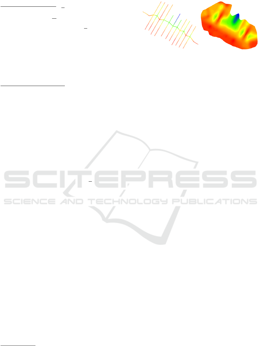
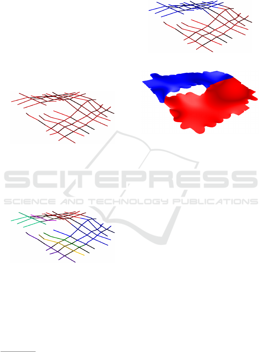
Figure 19: Example of real data: sparse polyline picking.
Figure 19 shows the input polylines as picked by
geologists on the survey. Many superposed zones will
be detected in the multivalued scan, leading to the in-
dexation of many sub-graphs in the index propagation
stage (see figure 20). The final sub-graph count will
not be excessive though, because of the merge step as
illustrated in figure 21.
Figure 20: Propagation of sub-graph indices in the con-
nected graph leads to the definition of 8 sub-graphs.
After conversion to heightmaps, envelope compu-
tation begins. This will lead to the definition of valid
envelope masks and neighbor data structures, used by
the gridding process. The resulting multivalued hori-
zon is depicted in figure 22.
5
Data size and density will be kept low for readability
though
Figure 21: After merging, sub-graph count is reduced to 2.
Figure 22: Following envelope computation and gridding, a
smooth multivalued surface is created.
5.2 Limits, Way Forward
The proposed interpolation chain is limited to poly-
lines. It would be an interesting feature to be able
to incorporate small heightmaps as well. Polylines
and heightmaps would be handled differently but with
the same spirit: it is indeed possible to detect super-
posed pixels, propagate per pixel and merge image
connected component before polylines are converted
to heightmaps.
Another way forward would be the handling of
faults during the gridding stage. Faults are the re-
sult of mechanical failure within a geological object.
These discontinuities can displace rock formations on
a wide range of distances, some largely visible even
at the seismic scale. Horizons can be for example cut
and displaced by faults – normal faults being one of
the primary source of multivalued horizons as pre-
sented in section 1. For this reason it makes sense
to prevent access to neighbor pixels on the opposite
side of a fault while gridding. This is a standard fea-
ture of current monovalued gridding implementations
in modern geophysics software, and would be appre-
ciated for multivalued horizons as well.
Beyond new features, many optimizations could
also be conducted in order to reduce the run-time
and memory footprint of the algorithmic chain. From
multi-grid schemes, multi-threading and compression
strategies to constraints for the sub-graph index prop-
agation, a lot of progress can be made to support ever
larger horizons. This is more relevant every day as
Reconstruction of Piecewise-explicit Surfaces from Three-dimensional Polylines
17

seismic resolution and survey size keep increasing
with technological advances in seismic reflection pro-
cesses.
6 STAGE OF THE RESEARCH
During this research project
6
we first searched for a
new model for multivalued horizons. Both qualitative
and quantitative comparisons have led to the construc-
tion of a piecewise-explicit surface representation, the
patch system model. An algorithm has then been pro-
posed in order to reconstruct a multivalued horizon
by interpolation from polylines, as exposed in this pa-
per. Our process has been validated by geologists that
will use it in order to interpret and reconstruct multi-
valued horizons, and has been shown to be robust
towards uncertainties in the input constraints (noisy
seismic signal leads to sparse and irregular picking).
Time will still be spent in several ways, first by op-
timizing the multivalued gridding pipeline. From new
features to implementation optimizations, the pro-
posed algorithm can be improved in many ways. Time
will also be spent to use the constructed multivalued
horizons for both display and processing. This will
lead to the development of triangulation algorithms
and the test of multivalued seismic attributes.
Our work on the handling of multivalued horizons
is innovative in the oil and gas industry, and will en-
hance the previously cumbersome process of multi-
valued horizon interpretation. Using our proposed
model and algorithms, it will be possible to pick, in-
terpolate, display and process a multivalued horizon
as a single object integrated in TOTAL’s geoscience
software Sismage CIG.
Moreover we provided a piecewise-explicit sur-
face model as well as a reconstruction scheme from
sparse polyline. This could be used in other appli-
cations where a complex surface must be represented
explicitly. Our work might for example help in devel-
oping new triangulation, surface processing or simu-
lation algorithms.
REFERENCES
Beckmann, N., Begel, H.-P., Schneider, R., and Seeger, B.
(1990). The R*-Tree: An Efficient and Robust Access
Method for Points and Rectangles. ACM Transactions
on Graphics, 19(2):322–331.
6
These advances were made possible thanks to a CIFRE
PhD collaboration between the the French ANRT, the
Gipsa-Lab and TOTAL SA
Bresenham, J. E. (1965). Algorithm for Computer Ccontrol
of a Digital Plotter. IBM Systems Journal, 4(1):25–30.
Briggs, I. C. (1974). Machine Contouring using Minimum
Curvature. Geophysics, 39:39–48.
Buluc, A., Meyerhenke, H., Safro, I., Sanders, P., and
Schulz, C. (2013). Recent Advances in Graph Par-
titioning. Lecture Notes in Computer Science, 9220.
Danielsson, E. (1980). Euclidian Distance Mapping. Com-
puter Graphics and Image Processing, 14:227–248.
Edelsbrunner, H., Kirkpatrick, D. G., and Seidel, R. (1983).
On the Shape of a Set of Points in the Plane. IEEE
Transactions on Information Theory, 29:551–559.
Grevera, G. J. (2004). Distance Transform Algorithms and
their Implementation and Evaluation. Technical re-
port, Saint Joseph’s University.
Hormann, K., Levy, B., and Sheffer, A. (2007). Mesh
Parameterization: Theory and Practice. Siggraph
Course Notes.
Kirkpatrick, D. G. and Seidel, R. (1986). The Ultimate Pla-
nar Convex Hull Algorithm. SIAM Journal on Com-
puting, 15:287–299.
Levoy, M. and Whitted, T. (1985). The Use of Points as
a Display Primitive. Technical report, University of
North Carolina at Chapel Hill, Computer Science De-
partment.
Meagher, D. J. R. (1982). Geometric modeling using
octree-encoding. Computer Graphics and Image Pro-
cessing, 19:129–147.
Russ, J. C. (1998). The Image Processing Handbook. CRC
Press.
Sadri, B. and Singh, K. (2014). Flow-complex-based Shape
Reconstruction from 3d Curves. ACM Transaction on
Graphics, 33(2):20:1–20:15.
Smith, W. H. F. and Wessel, P. (1990). Gridding with Con-
tinuous Curvature Splines in Tension. Geophysics,
55:293–305.
Treister, E. and Haber, E. (2016). A Fast Marching Algo-
rithm for the Factored Eikonal Equation. Journal of
Computational Physics, 324(C):210–225.
Walter, E. (2014). Numerical Methods and Optimization, a
Consumer Guide. Springer.
Zou, M., Holloway, M., Carr, N., and Ju, T. (2015).
Topology-Constrained Surface Reconstruction from
Cross-Sections. ACM Transactions on Graphics,
34(4):128:1–128:10.
DCGISTAM 2018 - Doctoral Consortium on Geographical Information Systems Theory, Applications and Management
18
