
Improved Cloud Partitioning Sampling for Iterative Closest Point:
Qualitative and Quantitative Comparison Study
Polycarpo Souza Neto, Nicolas S. Pereira and George A. P. Th
´
e
Department of Teleinformatic Engineering, Federal University of Ceara, Fortaleza,
Pici campus, Bl 725, Zip code 60455-970, Brazil
Keywords:
Computer Vision, Iterative Closest Point, Point Cloud Registration, Point Cloud Sampling.
Abstract:
In 3D reconstruction applications, an important issue is the matching of point clouds corresponding to different
perspectives of a given object in a scene. Traditionally, this problem is solved by the use of the Iterative Closest
point (ICP) algorithm. In view of improving the efficiency of this technique, authors recently proposed a
preprocessing step which works prior to the ICP algorithm and leads to faster matching. In this work, we
provide some improvements in our technique and compare it with other 4 variations of sampling methods
using a RMSE metric, an Euler angles analysis and a modification structural similarity (SSIM) based metric.
Our experiments have been carried out on four different models from two different databases, and revealed
that our cloud partitioning approach achieved more accurate cloud matching, in shorter time than the other
techniques. Finally we tested the robustness of the technique adding noise and occlusion, obtaining, as in the
other tests, superior performance.
1 INTRODUCTION
Efficient 3D reconstruction of indoor and outdoor en-
vironments is a hot research topic in many areas like
machine learning (Pan et al., 2017), in computer vi-
sion (Rodol
`
a et al., 2015), in photogrammetry (Zhang
and Lin, 2017) as well as for helping agriculture
through the use automated system for capturing 3D
data of plants and vegetation (Chaudhury et al., 2015)
and robotics (
´
Cesi
´
c et al., 2016) for tracking and de-
tection of elements in scenes. Also in manufactur-
ing industry (Toro et al., 2015) it may be seen as a
provider of innovative and efficient solutions for op-
timizing shop floor processes (Malamas et al., 2003),
what has been suggested especially in cases of colli-
sion avoidance (Cigla et al., 2017) in non-structured
scenarios and for safer human-machine interaction
(Gorecky et al., 2014), which ultimately may speed
up manufacturing processes.
In a few words, 3D reconstruction means data
fusion of images from different camera perspectives
and consists essentially on making partial descrip-
tions of a scene to merge into a scene representa-
tion as a whole. In the literature, this task has been
first solved by the Iterative Closest Point algorithm
(Besl and McKay, 1992). It is aimed at obtaining the
rigid transformation able to minimize the distance be-
tween two datasets, e.g. two acquired point clouds of
a given scene, allowing an integration of images ac-
quired from different camera position and orientation.
In general, ICP performs better when some data
preprocessing is carried out. In the literature, out-
liers removal (Weinmann, 2016) and undersampling
(Rodol
`
a et al., 2015) are typical issues; while the
former is important for good representation of the
rigid transformation pursued, latter influences com-
putational costs and its adoption is needed for sev-
eral reasons, as pointed out in (Rodol
`
a et al., 2015).
The sampling methods are useful discretization step
to produce data which is much easier to handle with
algorithms. Even if the surface is a triangular mesh,
sampling reduces the number of points to be repre-
sented, which may be required if the complexity of
the task is not linear or the clouds are large in size.
However, the goal of sampling is the selection of sur-
face points that are relevant with respect to the task
that is to be performed.
Authors recently proposed a sampling method
named cloud-partitioning ICP (CP-ICP) and it is re-
visited in this work, since important changes were
made to it (Pereira et al., 2015). We compared this
method with ICP as well as sampling methods based
on sampling. The techniques of comparison using
sampling were Random and Uniform Sampling. Uni-
Neto, P., Pereira, N. and Thé, G.
Improved Cloud Partitioning Sampling for Iterative Closest Point: Qualitative and Quantitative Comparison Study.
DOI: 10.5220/0006828500490060
In Proceedings of the 15th International Conference on Informatics in Control, Automation and Robotics (ICINCO 2018) - Volume 2, pages 49-60
ISBN: 978-989-758-321-6
Copyright © 2018 by SCITEPRESS – Science and Technology Publications, Lda. All rights reserved
49

form and random sampling variants were also stud-
ied in (Rusinkiewicz and Levoy, 2001). In the case
of Random Sampling, two variants were used, with
sampling of 50% and 70% of the data set. We have
compared the sampling methods quantitatively using
root mean squared error (RMSE) and Euler angles;
in addition, we adapt a form of quantitative evalua-
tion based on multi-view analysis of the registration
images, exposing these images to Structural Similar-
ity Index Measure (SSIM), proposing in (Wang et al.,
2004). Effects of adding noise and occlusion were
also investigated for some models, in order to provide
insight of robustness of the CP-ICP method under real
conditions of data acquisition.
The ICP implementation (in C++) of the Point
Cloud Library (PCL)(Holz et al., 2015) was adopted
here because it is widely used as benchmark by the
research community.
2 BASICS OF 3D MATCHING
The ICP algorithm was proposed in (Besl and McKay,
1992) and aims at finding a transformation that opti-
mizes a rotation and translation in two sets of data
(sets of line segments, implicit curves, sets of tri-
angles,implicit, parametric surfaces, point sets, etc.).
The algorithm uses one of the data sets as reference,
hereafter referred to as set and applies rotations and
translations to the other set, called here from now on
as input set, in order to minimize the following cost
function:
F(~q) =
1
N
N
∑
i=1
k~x
i
−(R~p
i
+ T ) k (1)
where:
• N=number of points;
• ~x
i
=i-th vector related to the target point cloud;
• ~p
i
=i-th vector related to the input point cloud;
• R= rotaxion matrix obtained from ICP;
• T= translation vector obtained from ICP.
The result achieved from the ICP algorithm is
the optimum rotation and translation between the two
datasets. Fig. 1 illustrates what happens after apply-
ing the ICP algorithm to point clouds. In the left, the
initial pose of the inputs and in the right, a successful
registration between the two point clouds.
Figure 1: Point cloud of Hammer model before (left) and af-
ter(right) submited from ICP algorith (Aleotti et al., 2014).
3 SAMPLINGS
3.1 Uniform Sampling
This ICP variant allows for crudely aligning one range
image to another and then invoking an algorithm that
snaps the position of one range image into great align-
ment to the other cloud. The implemented version
follows the description of (Turk and Levoy, 1994):
1. Find the nearest position on mesh A to each point
of mesh B;
2. Discard points out of range;
3. Delete pairs that are in a mesh boundary;
4. Find rigid transformation that minimizes weight-
ing distance to the square minimum between the
pairs of points.;
5. Run to converge;
6. Perform ICP on a more detailed mesh.
This ICP variant differs from classical ICP in sev-
eral ways. First, a distance boundary was added to
the nearest point to avoid combining any vertices B
i
from a mesh to a remote part otherwise than corre-
sponding to B
i
. This vertex B
i
of the mesh B may
be a part of the scanned object that has been not cap-
tured in mesh A. In (Turk and Levoy, 1994), it is said
that an excellent record is when the distance is ad-
justed to double the spacing between the reach points.
Limiting the distance between pairs of corresponding
points we performed step 2 (eliminating remote peers)
while searching for closest points in step 1.
ICINCO 2018 - 15th International Conference on Informatics in Control, Automation and Robotics
50
3.2 Random Sampling
Random sampling is a good downsampling tech-
nique, objectifying only to find internal points (Ma-
suda et al., 1996). We apply this technique to a first
image R
I
, and we draw a set of N
S
points of R
I
ran-
domly. One way to evaluate a probability of a good
sampling and considering a random sampling from a
probabilistic view point. Whatever epsilon a rejec-
tion of outliers by noise or occlusion, a probability of
choice inliers is 1 −ε. In addition, a probability of
choosing a subset with N
S
points that are all inliers
is (1 −ε). The N
T
value is a hair probability minus
a sub-sample being composed only of curious. The
equation that governs this method is shown below:
p(ε,N
S
,N
T
) = 1 −(1 −(1 −ε)
N
S
)
N
T
(2)
An example of random sampling can be seen in
(Nazem et al., 2014). In this paper, 70% of the data
sets are sampled before the registration process.
4 CLOUD PARTITIONING ICP
In line with that, recently authors proposed the cloud
partitioning approach to work prior the execution of
the ICP algorithm (CP-ICP). In the present version
of the algorithm, the idea behind the CP-ICP is to
separate the whole point cloud into smaller groups (k
groups in total) named hereafter subclouds, and then
repeat the registration process for every subcloud until
a stop criterion is found, as explained in section 4.1;
by doing that, we considerably reduce the amount of
computations because the point clouds are reduced in
size.
Originally (Pereira et al., 2015), ,the implementa-
tion did not consider the existence of a stop criterion,
what led to verification of k subclouds, and this some-
times proved to be unneccessary.The partitioning pro-
cess decreases the amount of data to be processed by
ICP in iteration, and the adoption of a stop criterion
prevents the algorithm from having to align among all
the subnets, stopping in the alignment of some sub-
cloud that has a lower RMSE than the stopping cri-
terion, which leads to time consuming and a guaran-
tee of a quality registration, although, within the set
of subnets there may be some where the alignment
is even better and the RMSE measurement confers
smaller values even of iteration where the algorithm
converge. Cutting of the point clouds in the CP-ICP
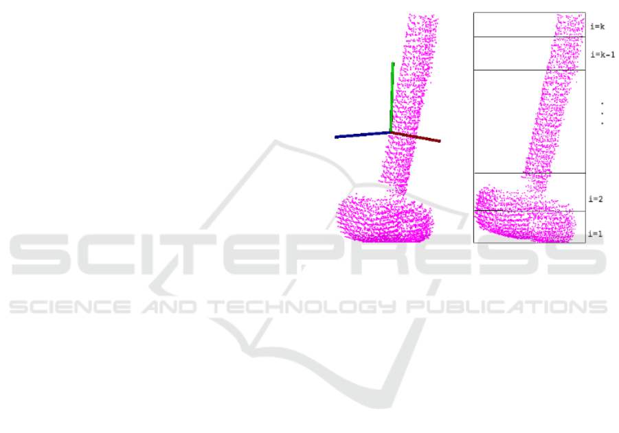
can be illustrated in Fig. 2, where after being iden-
tified where the cloud centroid is and its Z-axis, the
cuts are done in subclouds.
To get a better view on the above claiming, let N
X
and N
P
be the size of two clouds undergoing registra-
tion by the ICP. The cost for the closest point com-
putation in the classical ICP is O(N
X
N
P
) (Besl and
McKay, 1992), whereas using the partitioning into
subclouds makes the cost of the closest point compu-
tation to range from O(N
X
N
P
/k
2
) to kO(N
X
N
P
/k
2
).
This is because the stop criterion considered in the
current version, illustrated in the diamond of the flow-
chart in Fig. 3 may interrupt the whole matching at
any iteration from 1 to k.
Figure 2: The left side the identification of each axis of the
Hammer cloud in the coordinate system and to the right we
have after the identification of Z, the cut in k sub-clouds.
4.1 Sufficient Registration
Consider two point clouds: an input point cloud and a
target point cloud. The goal is to successfully perform
a registration procedure, which means matching the
input point cloud to the target one. To apply the CP-
ICP method, we perform the following steps:
1. Subdivide each dataset (input and target) into k
subclouds;
2. For each of the k iterations, solve the ICP algo-
rithm for a pair of subclouds. The correspondence
is checked between subclouds having the same in-
dex, and not one against all.
• Apply the achieved transformation to the initial
input point cloud (named from now on input post
ICP);
• The input post ICP is then compared to the target
point cloud, using RMSE error at each iteration;
• If the RMSE value achieved in a given iteration is
acceptable (stop criterion) the algorithm ends and
the wanted registration is outcome. This is a deci-
sion step and, as such, represented by diamond in
the flowchart of Fig. 3.
Improved Cloud Partitioning Sampling for Iterative Closest Point: Qualitative and Quantitative Comparison Study
51
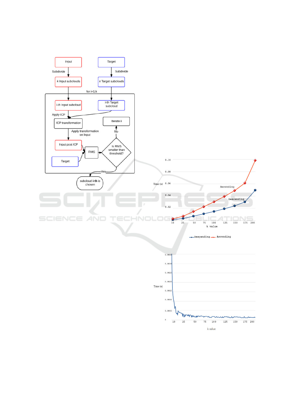
These steps are illustrated in the flow-chart of Fig. 3.
Figure 3: Fluxogram illustrating how the CP-ICP achieve a
sufficient registration.
Adopting a stop criterion is useful because it limits
the amount of correspondence checks between pairs
of subclouds, thus avoiding unneccessary repetitions
of ICP algorithm.
4.2 Tradeoff Between Solutions and
Time
Considering the CP-ICP method as shown in 3, one
can see that the more subclouds the more solutions
for transformation matrices are obtained, which is
good for finding an acceptable registration. However,
time consumption rises accordingly, what is a draw-
back, and reveals a tradeoff between the number of
solutions and the time consumption. That is why we
added a stop criterior to this algorithm. By doing that
at every correspondence check between pairs of sub-
clouds, we give the algorithm the ability to escape
and finish the matching whenever a good alignment
is found. Although in the current version the stop
criterion is determined a priori, this strategy has the
advantage to help reducing computational cost (com-
pared to the old published version).
To better explain the influence of the amount of
subclouds into the timing performance, we studied the
total elapsed time of the CP-ICP method, Fig. 4, as
well as the time spent in a single iteration, Fig. 5, for
different values of k. In figure 4 there are two curves;
they correspond to two different choices for the step
2 of the algorithm in section 4.1. Once the indexation
of the whole cloud and its grouping into k partitions
is done, the user must choose between ascending or
descending order to access the indexed subclouds in
the search for the best one. In some examples of the
database, the best subcloud is found near the begin-
ning of the for-loop, whereas in other data it takes the
whole spectrum of subclouds to be checked, slowing
down the CP-ICP running time. These two limit cases
are the ones represented by the lines of Fig. 4. In the
example of the figure, the downward direction choice
for accessing the i-th subcloud led to faster CP-ICP
execution.
Figure 4: The full time consumption.
Figure 5: The time consumption for a single iteration for
the Horse model.
ICINCO 2018 - 15th International Conference on Informatics in Control, Automation and Robotics
52
5 MATERIALS AND METHODS
5.1 Available Datasets
The performance of the proposed CP-ICP method was
evaluated from two different database. The first one
is a private database kindly provided by prof. Aleotti
in (Aleotti et al., 2014) and consists of point clouds of
several objects acquired from a 6DOF robot arm (Co-
mau SMART six) equipped with a two-finger parallel
gripper (Schunk PG-70) and a high-resolution range
laser scanner (SICK LMS 400), both mounted at the
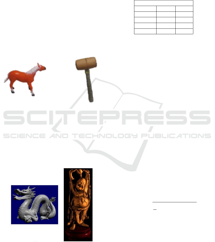
wrist of the robot arm. From this database we used
two models in our experiments, namely the Horse and
the Hammer models, illustrated in Fig. 6.
Figure 6: Objects from the database in (Aleotti et al., 2014).
The Horse model (left) and Hammer (right).
The perspectives available of those objects are la-
beled according to the angle of acquisition from the
sensor in the scene. For the Horse model we con-
sider the perspectives of 0
o
and 180
o
. For the Ham-
mer model we consider the perspectives of 0
o
and
45
o
. The second database is the Stanford 3D scanning
repository, illustrated in (Curless and Levoy, 1996),
which is a public database with several 3D models.
Figure 7: Objects from the database in (Curless and Levoy,
1996). The Dragon model (left) and Happy Buddha (right).
Similarly, the perspectives available of those ob-
jects are related to the acquisition angle.The image
acquired from the zero degree perspective is taken as
target cloud, whereas the one acquired from 24 de-
grees is considered as source cloud. Table 1.
Table 1: Various dataset size.
Number of points
Cloud Source Target
Horse 3335 3298
Hammer 1852 2024
Dragon 41841 34836
Buddha 78056 75582
5.2 Methodology
As pointed out earlier, the goal of this paper is
to introduce a new sampling method prior the ICP
algorithm (CP-ICP). To evaluate how it performs,
we compare CP-ICP with random sampling methods
(keeping up to 50% and 70% of the original point
cloud size) and also with a uniform sampling. In addi-
tion, we also considered the no-sampling case, which
is the classical ICP method of (Besl and McKay,
1992) as implemented in PCL. The ICP algorithm
then follows the sampling methods under study, and
the quality of the 3D registration is evaluated through
the Euler angles of the rotation matrix, by a metric
based on root mean squared (RMSE) error and, fi-
nally, by another metric based on an adaptation of
the structural similarity index (SSIM), to be discussed
next. In Fig. 8, this process is summarized.
5.3 Metrics for Matching Evaluation
We have adopted three different metrics to evalu-
ate the registration results and compare the sampling
methods. The first one is based on the root mean
squared error between the target point cloud and the
input point cloud after proper rotation correction.
The RMSE eror can be calculated by the following
formula:
RMSE =
s
1
N
N
∑
i=1
(min
x∈S
k y
i
−x k
2
)
2
, (3)
where S is an arbitrary surface and y1, ...,yN are
coordinate points in ℜ
3
, representing the surface ver-
tices or cloud points depending on a distance between
two surfaces or between a surface and a point in the
cloud.
The second metric is based on comparing the Eu-
ler angles from each transformation matrix obtained
through ICP. This can only be done to the Dragon and
Buddha models, since they have a ground truth.
Improved Cloud Partitioning Sampling for Iterative Closest Point: Qualitative and Quantitative Comparison Study
53
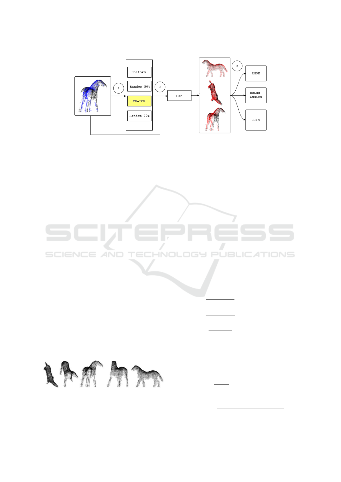
Figure 8: Methodology adopted to compare the sampling methods. In (1) the clouds go through a sampling process, in (2)
the ICP is applied to perform the alignment, in (3) the outputs of the registry go through the evaluation of the registry quality
metrics.
The rotation matrix can be defined by R, and the
results of the Euler angles are obtained by the resolu-
tions of the trigonometric products contained therein
(Corke, 2017).
R =
c
y
c
z
c
x
s
x
s
y
−c
x
s
z
s
x
s
z
+ c
x
c
z
s
y
c
y
s
z
c
x
c
z
+ s
x
s
y
s
z
c
x
s
y
s
z
−c
z
s
x
−s
y
c
y
s
x
c
x
c
y
(4)
where: c
x
=cos(α), c
y
=cos(β), c
z
=cos(γ),
s
x
=sen(α), s
y
=sen(β) and s
z
=sen(γ).
The last metric is based on the SSIM index, which
is a traditional approach to measure image quality. It
is also a method applied to identify similarity between
two gray-scale images, where one of them is treated
as a reference image. The SSIM index is an image
quality metric which assess three characteristics of an
image: the contrast, luminance and structure, each of
them being calculated from statistical parameters of
the input images.
In this paper, we adapt a method which uses the
SSIM index to perform the comparison between 3D
models by creating 2D images of different perspec-
tives of each model and comparing them using the
SSIM index. To illustrate how the method is made
suitable for 3D, we start with the registration result as
obtained by the CP-ICP for the Horse model from five
perspectives, in Fig. 9.
Figure 9: The five perspectives for the CP-ICP registration
of the Horse model.
The use of the SSIM technique here relies on gen-
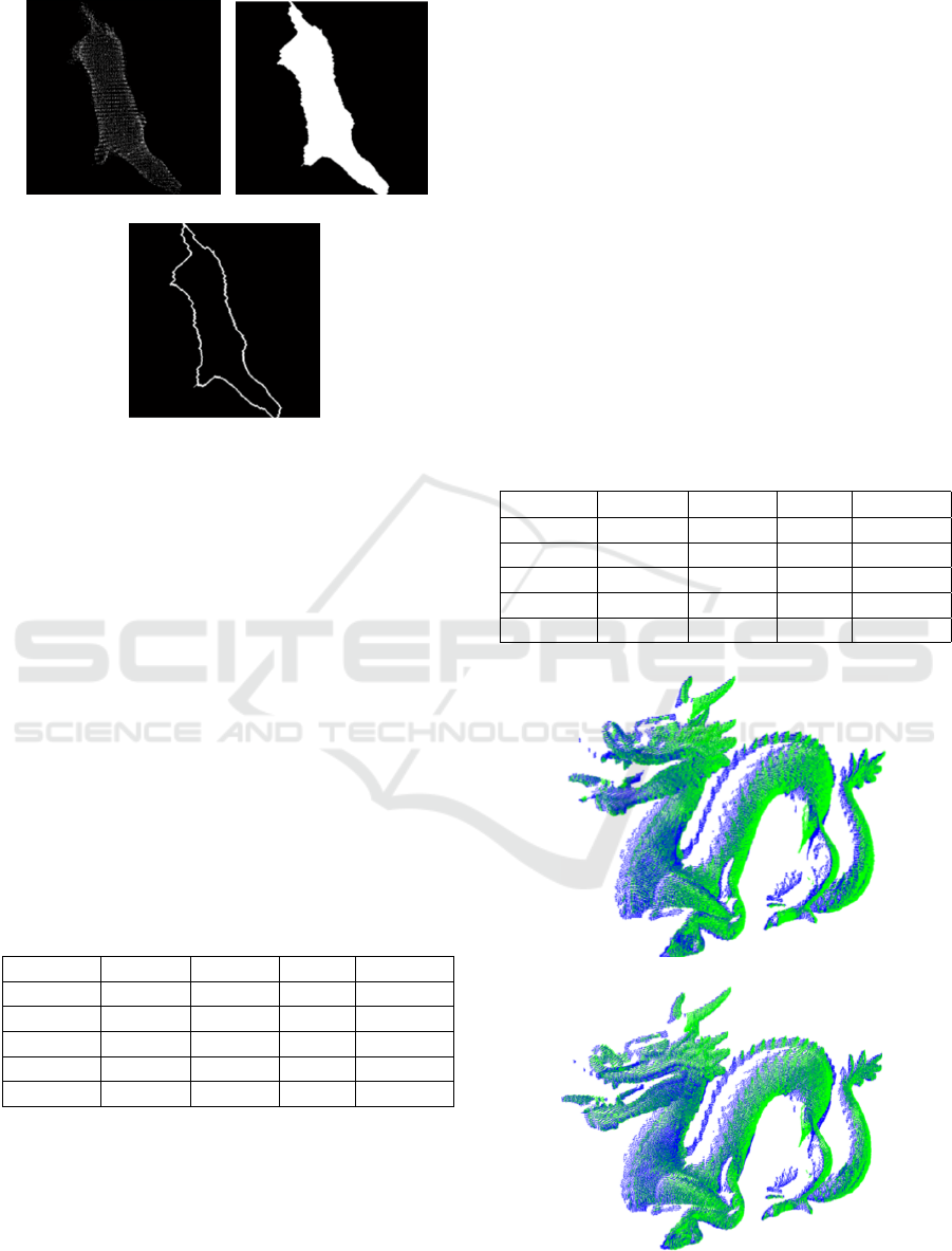
erating three images for each perspective: dot pat-
tern image, full image and edge image, each one
with 512x512 resolution. We got the dot pattern im-
age after a quantization of point dataset as visualized
from one of the perspectives, whereas the others are
achieved from morphological transformations applied
in the dot pattern image. Fig. 10(a), 10(b) and 10(c)
show this set of images using as example the first per-
spective of 9. Fig. 10(b) and 10(c) are respectively
the images after dilation and border extraction (Soille,
2003).
Dilation depicted in Fig.10(b) is the result of prob-
ing and expanding (until background is found) the
inner of the input image from a structuring element.
Border extraction then follows this dilation by means
of subtracting it from the input image.
According to (Wang et al., 2004), the functions
l(a, b), c(a,b) and s(a,b) are then defined as:
l(a, b) =
2µ
a
µ
b
+C
1
µ
2
a
+ µ
2
b
+C
1
|C
1
= (K
1
L)
2
,K
1
1 (5)
c(a,b) =
2σ
a
σ
b
+C
2
σ
2
a
+ σ
2
b
+C
2
|C
2
= (K
2
L)
2
,K
2
1 (6)
s(a,b) =
2σ
ab
+C
3
σ
a
σ
b
+C
3
|C
3
= (K
3
L)
2
,K
3
1 (7)
Where µ
a
and µ
b
are the pixel intensities of each im-
age, σ
a
and σ
b
are the standard deviations, C
1
, C
2
and
C
3
are constants added to each term, L is the pixel
range (255 for 8-bit grayscale images, e.g.) and K
1
,K
2
and K
3
are constants less than unity. In addition, σ
ab
is calculated as:
σ
ab
=
1
N
a
−1
N
a
∑
i=1
(a
i
−µ
a
)(b
i
−µ
b
) (8)
Finally, the metric takes the form presented below:
SSIM(a, b) =
(2µ
a
µ
b
+C
1
)(2σ
ab
+C
2
)
(µ
2
a
+ µ
2
b
+C
1
)(σ
2
a
+ σ
2
b
+C
2
)
(9)
ICINCO 2018 - 15th International Conference on Informatics in Control, Automation and Robotics
54
(a) (b)
(c)
Figure 10: The three kind of images generated for each per-
spective of each model. In (a) dot pattern image, in (b) full
image (dilated), in (c) edge image (border extraction).
6 RESULTS
6.1 Elapsed Time
Table 2 synthetizes the time performance of the
various sampling approaches; as it is clear from
the results, the proposed CP-ICP sampling method
achieved top performance for each 3D model stud-
ied. Such a good performance of the proposed ap-
proach somewhat confirms the expectations about the
reduced computational efforts of the cloud matching
algorithm, as mentioned in Section 4.
Table 2: Time comparision in seconds between sampling
methods.
Buddha Dragon Horse Hammer
CP-ICP 0.62 0.22 0.048 0.025
ICP 17.68 7.40 0.41 0.37
Rnd. 50 17.85 4.01 0.36 0.19
Rnd. 70 18.72 5.82 0.43 0.26
Uniform 14.27 4.39 0.58 0.35
These numbers are impressive because they em-
phasize that the proposed approach is faster than the
benchmark, and the impact into this particular re-
search field is therefore evident.
6.2 RMSE Metrics
As explained earlier, in addition to the analysis of the
performance regarding the time required to complete
the registration procedure we also looked for a quan-
titative measure of the matching quality. In this paper
we suggest to use, in a first moment, the root mean
squared error between the target point cloud for the
ICP algorithm and the input post ICP.
From Table 3, we can see that the CP-ICP method
and the other approaches perform similarly. To illus-
trate with images what these numbers express, Fig.
11 brings the cloud matching for the Dragon model,
which is a big-size point cloud. In Fig. 11(a) we can
see the ICP registration (with no sampling), whereas
the matching using the CP-ICP method is plotted in
Fig. 11(b).
Table 3: RMSE evaluated after the ICP with each technique.
The numbers are multiplied by 10
2
.
10
−2
Buddha Dragon Horse Hammer
CP-ICP 0.26 0.18 0.98 0.60
ICP 0.24 0.18 0.97 0.57
Rnd. 50 0.24 0.19 1.08 0.60
Rnd. 70 0.24 0.18 1.05 0.59
Uniform 0.24 0.19 0.97 0.58
(a)
(b)
Figure 11: Registration results for the Dragon models. In a)
the result obtained with the classical ICP In b) the CP-ICP.
Improved Cloud Partitioning Sampling for Iterative Closest Point: Qualitative and Quantitative Comparison Study
55
6.3 Euler Angles Analysis
As an additional result for the quantitative analysis of
the point cloud matching, in Table 4 and 5 the trans-
formation matrix is represented by its Euler angles.
The total error is the sum of the Z-, Y- and X- axis
minus the ground-truth.
This was made only for the Dragon and Buddha
models because the ground truth is known to be 24
o
around Z axis.
Table 4: Euler angle of Happy Buddha model.
Buddha
In degree Z Y X Total error
CP-ICP 24.01 -0.13 -0.14 0.26
ICP 18.98 0.54 -0.81 5.29
Rnd. 50 19.33 0.37 -0.82 5.12
Rnd. 70 19.13 0.42 -0.79 5.24
Uniform 19.11 0.30 -0.75 5.34
Table 5: Euler angle of Dragon model.
Dragon
In degree Z Y X Total error
CP-ICP 23.77 0.08 0.24 0.09
ICP 23.91 0.16 0.23 0.30
Rnd. 50 23.88 0.14 0.23 0.25
Rnd. 70 23.89 0.17 0.24 0.30
Uniform 23.89 0.15 0.24 0.28
Once again, the CP-ICP was shown to be supe-
rior also from a quantitative point of view. The reader
should especially note the column for the Z axis of
the Buddha model. Besides that, we can observe the
column representing the total error, which is the sum
of the angles in the three axes: while the estimates
from the other techniques deviate of about 5 degrees,
the CP-ICP error approches zero. The success of the
CP-ICP on finding the Euler angles which best repre-
sent the relative orientation between the point clouds
relies on the fact that our algorithm is able to iden-
tify the region of the 3D model which preserves the
most important points describing the rigid transfor-
mation searched. Unlike ICP, which searches for op-
timal transformation in the entire source cloud,
in CP-ICP this is done one sub-cloud at a time, in
a ”light fashion.
6.4 SSIM-based Metrics
Tables 6 to 9 show the analysis of the five perspectives
of each of the 3D models studied, using metrics based
on SSIM, and represent average values between the
perspectives. Tables 6 and 7 are related to the Bud-
dha and Dragon models (largest data sets), while 8
and 9 are related to the Hammer and Horse models
(small datasets). As shown in Tables 6 and 7, dif-
ferent to what has been seen so far, the various meth-
ods performs better in the Buddha model according to
the proposed metrics. In the comparision between the
sampling approaches, once again CP-ICP beats them
all.
The results obtained for the evaluation through the
SSIM can be seen in the tables below, with the best
overall results, that is, the averages of all dot pattern,
full and contour views highlighted in bold. It is seen
that, in all cases, the best mean was CP-ICP.
Table 6: SSIM based comparison for the Happy Buddha
model.
Buddha
Dot Full Contour Mean
CP-ICP 0.884 0.941 0.982 0.936
ICP 0.822 0.947 0.965 0.911
Rnd. 50 0.869 0.947 0.979 0.911
Rnd. 70 0.872 0.947 0.975 0.932
Uniform 0.876 0.953 0.975 0.935
Table 7: SSIM based comparison for the Dragon model.
Dragon
Dot Full Contour Mean
CP-ICP 0.568 0.683 0.967 0.740
ICP 0.570 0.621 0.900 0.697
Rnd. 50 0.583 0.644 0.902 0.716
Rnd. 70 0.570 0.621 0.902 0.698
Uniform 0.576 0.632 0.916 0.708
Table 8: SSIM based comparison for the Hammer model.
Hammer
Dot Full Contour Mean
CP-ICP 0.962 0.936 0.999 0.966
ICP 0.931 0.921 0.999 0.950
Rnd. 50 0.940 0.935 0.998 0.958
Rnd. 70 0.938 0.934 0.999 0.957
Uniform 0.941 0.938 0.992 0.960
Table 9: SSIM based comparison for the Horse model.
Horse
Dot Full Contour Mean
CP-ICP 0.902 0887 0.999 0.929
ICP 0.901 0.889 0.996 0.929
Rnd. 50 0.892 0.891 0.999 0.928
Rnd. 70 0.892 0.843 0.999 0.928
Uniform 0.891 0.889 0.999 0.926
In general, for the four point cloud models used,
the SSIM metrics agrees with the other ones and con-
firms the superior matching quality of the CP-ICP.
ICINCO 2018 - 15th International Conference on Informatics in Control, Automation and Robotics
56
Overall, these tables and figures reveal that the CP-
ICP approach presented the best performance for all
point cloud models.
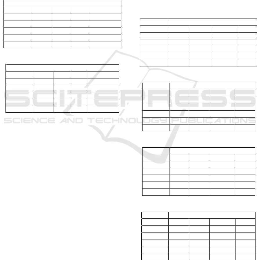
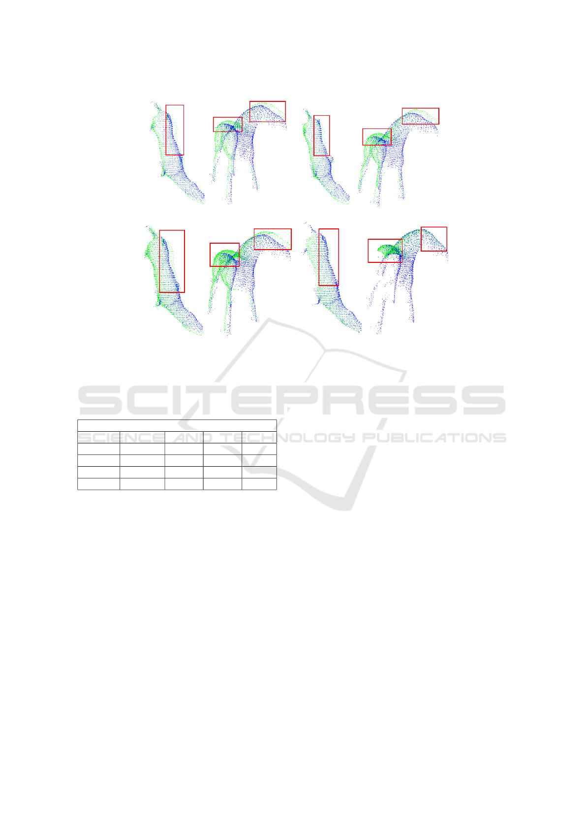
For the sake of illustration, Fig. 12 brings the reg-
istration results: a)using the CP-ICP; b) using ran-
dom sampling with 70% of the points and c) using
the ICP with no sampling. The highlighted regions
of 12(a) reveals that the registration following cloud
partitioning approach achieved a better qualitative re-
sult, though quantitatively the ICP method softly beat
it (see Table 3).
(a)
(b)
(c)
Figure 12: Comparison of the registration results for the
Horse model. In a) the registration for the CP-ICP b) the
registration result for the random 70% sampling and in c)
the registration result for the ICP with no samling.
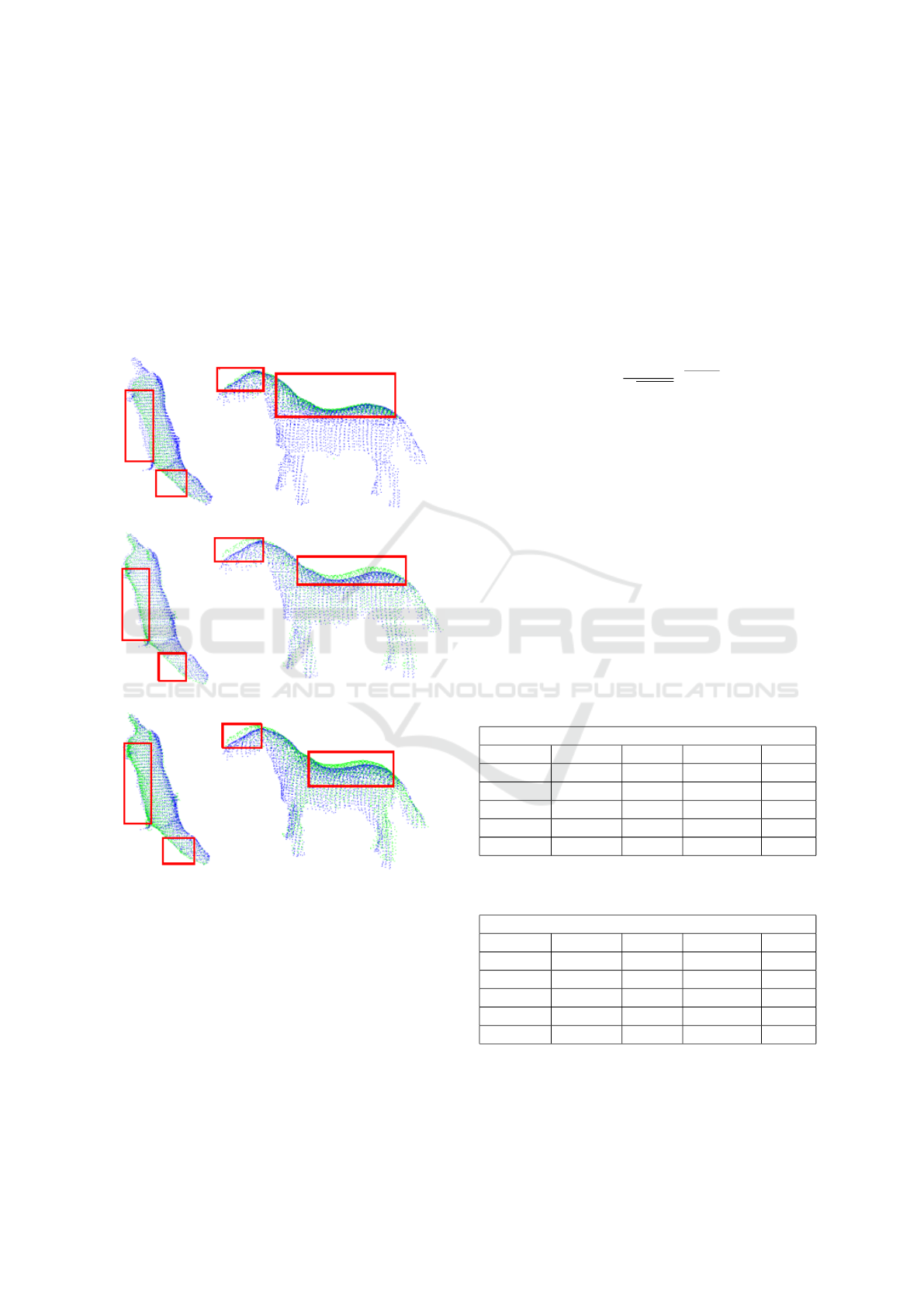
Finally, in Fig. 13 the registration results for the
Buddha are plotted. For the Buddha model, we can
clearly see that the CP-ICP result presents itself as the
best registration, as denoted in the marked regions in
13(f)
7 ROBUSTNESS TO NOISE AND
OCCLUSION
In (Masuda and Yokoya, 1995), a robust noise and
occlusion technique is discussed, which motivated ex-
periments to test the robustness of our technique. To
accomplish with that, we considered adding gaussian
noise and subjecting the clouds to occlusion. Only
the Buddha and Dragon models were considered here.
The probability density function p of a Gaussian ran-
dom variable z is given by:
p
G
(z) =
1
√
σ ∗2π
e
−(z−µ)
2
2σ
2
(10)
where z represents the grey level, µ the mean value
and σ the standard deviation. In this case σ = 0.001.
The results are summarized in Tables 10 and 11,
which bring the various metric adopted and the dif-
ferent sampling approaches at a glance. We can ob-
serve the best performance is achieved by CP-ICP,
which approached better the 24 degrees Z-axis rota-
tion of the ground truth in extremely short time. Er-
rors regarding the other axis follow analogously and
are omitted for brevity. In addition to the observation
of the tables, we can make a brief visual inspection
in Fig. 14(e), looking at the Buddha’s feet. We can
say that the regions between the clouds of origin and
target overlap perfectly when registration follows CP-
ICP.
Table 10: Table with comparison metrics for the Buddha
model for registration with Gaussian noise addition.
Buddha
Time (s) RMSE Angle (
o
) SSIM
CP-ICP 0.67 0.19 21.30 0.901
ICP 15.32 0.21 15.71 0.897
Rnd.50 7.44 021 16.02 0.889
Rnd.70 10.71 0.20 16.00 0.888
Uniform 10.62 0.20 16.01 0.889
Table 11: Table with comparison metrics for the Dragon
model for registration with Gaussian noise addition.
Dragon
Time (s) RMSE Angle (
o
) SSIM
CP-ICP 0.18 0.16 23.97 0.778
ICP 7.03 0.17 23.59 0.769
Rnd.50 4.17 0.18 23.59 0.765
Rnd.70 5.58 0.17 23.58 0.769
Uniform 4.12 0.18 23.58 0.756
The robustness to occlusion was studied from the
Horse model. One of the main problems of project-
ing the 3D scene to the image plane is occlusion -
each object blocks the view of others behind it (Huang
Improved Cloud Partitioning Sampling for Iterative Closest Point: Qualitative and Quantitative Comparison Study
57
(a) (b) (c)
(d) (e) (f)
Figure 13: Comparison of the registration results for the Buddha model. In a) the image of the foot of the Buddha, in b)the
registration result for the random 50% sampling and in c) the registration result for the random 70% sampling and in d) the
registration result for the uniform sampling and in e) the registration result for the ICP with no samling and finally in f)the
registration result of use CP-ICP method.
(a) (b) (c) (d)
(e)
Figure 14: Comparison of registration results for the Buddha model with Gaussian noise of standard deviation 0.001. In a)
the registration result for the random 50% sampling and in b) the registration result for the random 70% sampling and in c)
the registration result for the uniform sampling and in d) the registration result for the ICP with no samling and finally in e)the
registration result of use CP-ICP method.
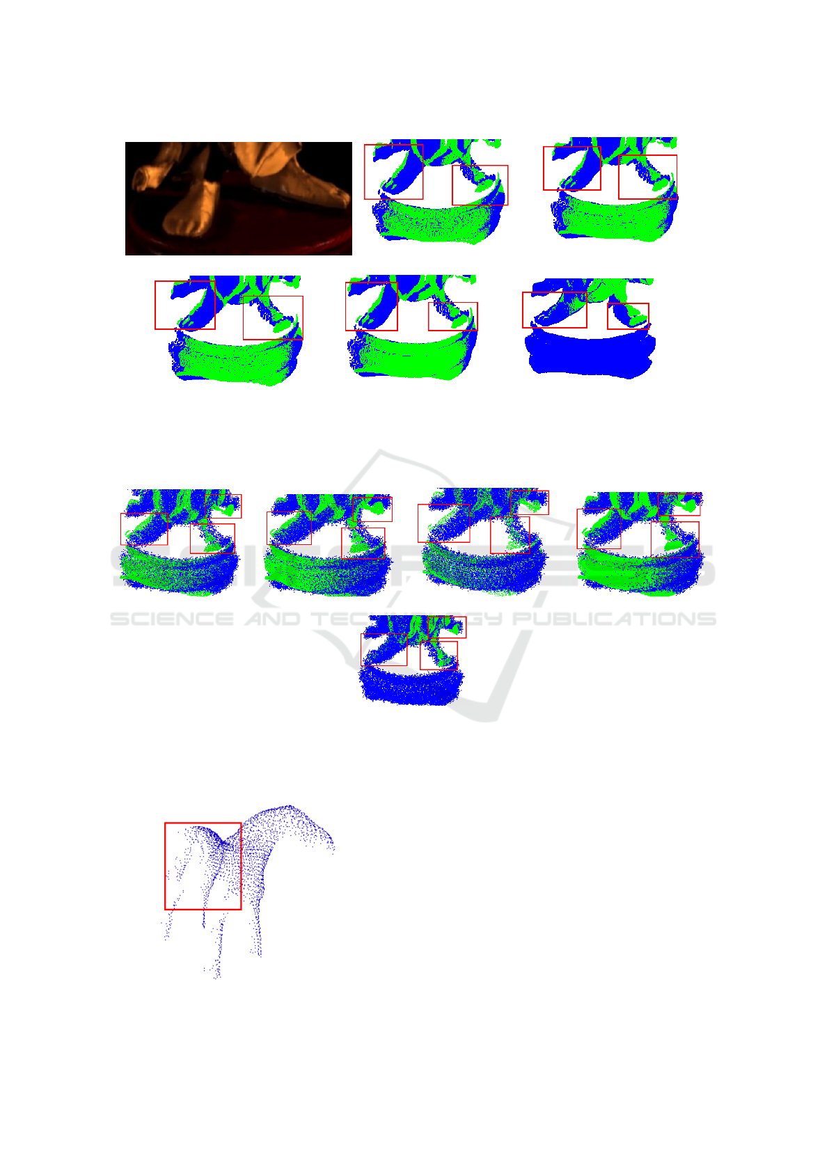
Figure 15: Horse model occluded.
et al., 2017). The occlusion can be caused by the
omission of the vision of a given mass of points due
to the presence of another object in the front, or can
be caused by a rotation of the object itself. For the
latter case, we call it self-occlusion.
In our experiment, a local maximum filter of the
PCL itself was used to make localized removal of
points in the back of the Horse, causing the lateral
points at left to disappear almost completely. The
sketch of it can be seen in Fig. 15. Despite of that
image perturbation, CP-ICP outperformed the various
sampling methods.
ICINCO 2018 - 15th International Conference on Informatics in Control, Automation and Robotics
58
(a) (b)
(c) (d)
Figure 16: Results for the Horse model with partial occlusion of points. In a) the registration result for the random 50%
sampling and in b) the registration result for the random 70% sampling and in c) the registration result for the ICP with no
samling and finally in e)the registration result of use CP-ICP method.
Table 12: Results of registration of Horse model apllying
occlusion.
Horse
Time (s) RMSE Angle SSIM
CP-ICP 0.052 1.37 180.00 0.943
ICP 0.94 1.32 177.56 0.939
Rnd.50 0.53 1.42 177.17 0.940
Rnd.70 0.74 1.41 177.34 0.943
Observing the result in the table 12, the register
with the CP-ICP presents better results: it completely
found the ground truth and, in addition, reached the
highest SSIM. For what concerns the RMSE measure,
it fluctuated very little amongst the sampling methods
and, hence, it can’t be used as a faithful comparison
metric in these cases.
Robustness of CP-ICP to added noise is related to
its ability to keep the original data of the point clouds;
indeed, not even a single point is lost when sub-clouds
are checked for correspondence. Unlikely, sampling
approaches lead to loss of input data (in some case
it leads to pseudodata generation), and consequently
noise gets more important, thus biasing the ICP to
find erroneous correspondences.The success of the
CP-ICP technique when dealing with self-occlusion
may be associated to the partitioning itself: since we
search for correspondences between sub-clouds, even
under partial occlusion scenario there are many sub-
clouds in which the input data is fully preserved and,
as such, are useful for correspondence search.
8 CONCLUSIONS
In this paper, a pre-processing method was presented
for registration along with ICP. The method is com-
pared with other four techniques using an RMSE met-
ric, Euler angles, and one metric adapted from SSIM.
The results show that, in comparison to the other
methods, author’s approach provided a better regis-
tration in shorter times. This technique also presented
robustness to data corruption by gaussian noise and
subject to occlusion, as well. This is therefore, a
promising and useful preprocessing step to use with
ICP variants in real time applications of 3D mod-
elling.As future work, we will make the algorithm
fully automatic, as well we will implement the align-
ment of one sub-cloud against all.
ACKNOWLEDGEMENTS
The authors are grateful to Professor Marques for lab
facilities and agency FUNCAP for the financial sup-
port.
Improved Cloud Partitioning Sampling for Iterative Closest Point: Qualitative and Quantitative Comparison Study
59

REFERENCES
Aleotti, J., Rizzini, D. L., and Caselli, S. (2014). Percep-
tion and grasping of object parts from active robot ex-
ploration. Journal of Intelligent & Robotic Systems,
76(3-4):401–425.
Besl, P. J. and McKay, N. D. (1992). Method for regis-
tration of 3-d shapes. In Sensor Fusion IV: Control
Paradigms and Data Structures, volume 1611, pages
586–607. International Society for Optics and Photon-
ics.
´
Cesi
´
c, J., Markovi
´
c, I., Juri
´
c-Kavelj, S., and Petrovi
´
c, I.
(2016). Short-term map based detection and tracking
of moving objects with 3d laser on a vehicle. In In-
formatics in Control, Automation and Robotics, pages
205–222. Springer.
Chaudhury, A., Ward, C., Talasaz, A., Ivanov, A. G., Huner,
N. P., Grodzinski, B., Patel, R. V., and Barron, J. L.
(2015). Computer vision based autonomous robotic
system for 3d plant growth measurement. In Com-
puter and Robot Vision (CRV), 2015 12th Conference
on, pages 290–296. IEEE.
Cigla, C., Brockers, R., and Matthies, L. (2017). Image-
based visual perception and representation for colli-
sion avoidance. In IEEE International Conference on
Computer Vision and Pattern Recognition, Embedded
Vision Workshop.
Corke, P. (2017). Robotics, Vision and Control: Funda-
mental Algorithms In MATLAB
R
Second, Completely
Revised, volume 118. Springer.
Curless, B. and Levoy, M. (1996). A volumetric method for
building complex models from range images. In Pro-
ceedings of the 23rd annual conference on Computer
graphics and interactive techniques, pages 303–312.
ACM.
Gorecky, D., Schmitt, M., Loskyll, M., and Z
¨
uhlke, D.
(2014). Human-machine-interaction in the industry
4.0 era. In Industrial Informatics (INDIN), 2014 12th
IEEE International Conference on, pages 289–294.
IEEE.
Holz, D., Ichim, A. E., Tombari, F., Rusu, R. B., and
Behnke, S. (2015). Registration with the point cloud
library: A modular framework for aligning in 3-d.
IEEE Robotics & Automation Magazine, 22(4):110–
124.
Huang, P., Cheng, M., Chen, Y., Luo, H., Wang, C., and Li,
J. (2017). Traffic sign occlusion detection using mo-
bile laser scanning point clouds. IEEE Transactions
on Intelligent Transportation Systems, 18(9):2364–
2376.
Malamas, E. N., Petrakis, E. G., Zervakis, M., Petit, L., and
Legat, J.-D. (2003). A survey on industrial vision sys-
tems, applications and tools. Image and vision com-
puting, 21(2):171–188.
Masuda, T., Sakaue, K., and Yokoya, N. (1996). Registra-
tion and integration of multiple range images for 3-d
model construction. In Pattern Recognition, 1996.,
Proceedings of the 13th International Conference on,
volume 1, pages 879–883. IEEE.
Masuda, T. and Yokoya, N. (1995). A robust method for
registration and segmentation of multiple range im-
ages. Computer vision and image understanding,
61(3):295–307.
Nazem, F., Ahmadian, A., Seraj, N. D., and Giti, M. (2014).
Two-stage point-based registration method between
ultrasound and ct imaging of the liver based on icp
and unscented kalman filter: a phantom study. Inter-
national journal of computer assisted radiology and
surgery, 9(1):39–48.
Pan, J., Chitta, S., and Manocha, D. (2017). Probabilistic
collision detection between noisy point clouds using
robust classification. In Robotics Research, pages 77–
94. Springer.
Pereira, N. S., Carvalho, C. R., and Th
´
e, G. A. (2015). Point
cloud partitioning approach for icp improvement. In
Automation and Computing (ICAC), 2015 21st Inter-
national Conference on, pages 1–5. IEEE.
Rodol
`
a, E., Albarelli, A., Cremers, D., and Torsello, A.
(2015). A simple and effective relevance-based point
sampling for 3d shapes. Pattern Recognition Letters,
59:41–47.
Rusinkiewicz, S. and Levoy, M. (2001). Efficient variants
of the icp algorithm. In 3-D Digital Imaging and Mod-
eling, 2001. Proceedings. Third International Confer-
ence on, pages 145–152. IEEE.
Soille, P. (2003). Morphological image analysis: princi-
ples and applications. Springer Science & Business
Media.
Toro, C., Barandiaran, I., and Posada, J. (2015). A per-
spective on knowledge based and intelligent systems
implementation in industrie 4.0. Procedia Computer
Science, 60:362–370.
Turk, G. and Levoy, M. (1994). Zippered polygon meshes
from range images. In Proceedings of the 21st an-
nual conference on Computer graphics and interac-
tive techniques, pages 311–318. ACM.
Wang, Z., Bovik, A. C., Sheikh, H. R., and Simoncelli, E. P.
(2004). Image quality assessment: from error visi-
bility to structural similarity. IEEE transactions on
image processing, 13(4):600–612.
Weinmann, M. (2016). Outlier removal and fine registra-
tion. In Reconstruction and Analysis of 3D Scenes,
pages 84–85. Springer.
Zhang, J. and Lin, X. (2017). Advances in fusion of optical
imagery and lidar point cloud applied to photogram-
metry and remote sensing. International Journal of
Image and Data Fusion, 8(1):1–31.
ICINCO 2018 - 15th International Conference on Informatics in Control, Automation and Robotics
60
