Parameter Identiﬁcation in Cyclic Voltammetry

of Alkaline Methanol Oxidation

Tanja Clees

, Igor Nikitin

, Lialia Nikitina

, Sabine Pott

, Ulrike Krewer

and Theresa Haisch

Fraunhofer Institute for Algorithms and Scientiﬁc Computing, Sankt Augustin, Germany

Institute of Energy and Process Systems Engineering, Technical University Braunschweig, Germany

Keywords:

Complex Systems Modeling and Simulation, Non-linear Optimization, Parameter Identiﬁcation, Application

in Electrochemistry.

Abstract:

Alkaline methanol oxidation is an electrochemical process, perspective for the design of efﬁcient high energy

density fuel cells. The process involves a large number of elementary reactions, forming a complex reaction

graph, and it is described by a system of non-linear differential equations of high order. The purpose of param-

eter identiﬁcation is a reconstruction of reaction constants in this model on the basis of available experimental

data. Cyclic voltammetry, a measurement of dynamical current-voltage characteristic of the cell, is especially

suitable for analysis of electrochemical kinetics. In this paper we present several approaches for parame-

ter identiﬁcation in cyclic voltammetry of alkaline methanol oxidation. With the aid of global optimization

methods and interactive parameter study we ﬁnd four islands of solutions in parameter space, correspond-

ing to different chemical mechanisms of the process. The main features of solutions are discussed and the

reconstructed reaction constants are presented.

1 INTRODUCTION

Direct fuel cells are attractive portable energy

sources, serving as converters of chemical energy

to the electric one, with a possibility to reﬁll the

reagents. Alkaline methanol oxidation uses com-

monly available components and allows to reduce the

costs for production and operation of the cells. The

detailed description of this chemical process includes

a large number of reactions, multiple intermediates,

leading to a mathematical model with many unknown

parameters (Krewer et al., 2011; Krewer et al., 2006;

Beden et al., 1982).

For parameter identiﬁcation different types of ex-

periments are used (Ciucci, 2013; Gamry Instru-

ments, 2018). Some of them measure stationary

current-voltage proﬁles of the cell, others use a lin-

earization near the stationary point and scan a re-

sponse of the cell to harmonic oscillations in a large

range of frequencies. In our previous paper (Clees

et al., 2017) we have presented the methods for pa-

rameter identiﬁcation in this type of measurements.

The main difﬁculty here is that the stationary state

in the considered process is hard to reach experimen-

tally. Our laboratory measurements show that even if

one leaves the cell under ﬁxed voltage for six hours, it

does not reach a steady current. A presumable reason

is a gradual poisoning of the electrode with intermedi-

ates or byproducts of reactions, characteristic for the

measurements of this type.

In this paper, differently from (Clees et al., 2017),

the measurement method is used, not assuming the

presence of the stationary state. Cyclic voltammetry

(Bard and Faulkner, 2000) is an experimental setup,

where the cell is subjected to a saw-like voltage varia-

tion of high amplitude. These voltage variations clean

up the electrode during every period, in this way pre-

venting the electrode poisoning. On the side of pa-

rameter identiﬁcation, however, the problem becomes

more difﬁcult, since one needs to integrate numeri-

cally stiff non-linear differential equations, instead of

just testing the linear response of the system.

In general, parameter identiﬁcation uses a version

of non-linear least square method (Press et al., 1992;

Strutz, 2016) to ﬁt the experimental data with the

mathematical model. One can also take into account

any equality or inequality constraints by the meth-

ods of non-linear programming, e.g., interior point

method (W

achter and Biegler, 2006). These methods

ﬁnd only a local optimum and should be enhanced by

global strategies to ﬁnd all relevant solutions. One

possibility is an interactive exploration of solution

Clees, T., Nikitin, I., Nikitina, L., Pott, S., Krewer, U. and Haisch, T.

Parameter Identiﬁcation in Cyclic Voltammetry of Alkaline Methanol Oxidation.

DOI: 10.5220/0006832002790288

In Proceedings of 8th International Conference on Simulation and Modeling Methodologies, Technologies and Applications (SIMULTECH 2018), pages 279-288

ISBN: 978-989-758-323-0

279

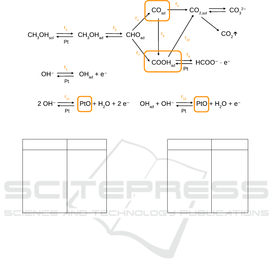
Figure 1: Reaction graph. Orange frames indicate possible locations of weakly coupled reagents.

Table 1: Numeration of variables and constants.

Variables Constants

−

CHO

COOH

PtO

space using metamodeling with radial basis functions

(Nikitin et al., 2012; Clees et al., 2014a; Clees et al.,

2014b). For the problem in hand, however, solutions

occupy thin subsets of parameter space. Also, the de-

pendence of model response on parameters includes

rapidly growing exponential terms, too non-linear to

be caught with radial basis functions. Instead of in-

terpolating the response, one can directly solve the

differential equations, provided that the integrator is

sufﬁciently fast. Interactive exploration can be also

enhanced with standard global optimization methods

ack, 1996; Ilonen et al., 2003; Otten and van Gin-

neken, 1989), including genetic algorithms, differen-

tial evolution, simulated annealing, etc.

In this paper we use a combination of automatic

global methods and interactive parameter study. In

Section 2 we present the mathematical model behind

alkaline methanol oxidation. In Section 3 the experi-

mental measurements are described. In Section 4 the

details on parameter identiﬁcation methods are given.

Section 5 presents the obtained results.

Table 2: Model constants.

Constant, units Value

F, C/mol 9.649 · 10

R, J/(K mol) 8.314

A, m

2.376 · 10

−5

, F 1.899 · 10

−4

act

, mol/m

8.523 · 10

−5

α 0.5

2 ALKALINE METHANOL

OXIDATION

Considering alkaline methanol oxidation processes,

we use the list of reactions from our previous work

(Clees et al., 2017):

: OH

−

+ Pt ↔ OH

+ e

−

: CH

OH + Pt ↔ CH

: CH

+ 3OH

↔ CHO

+ 3H

: CHO

+ OH

→ CO

+ H

: CO

+ 2OH

→ CO

+ H

O + 2Pt

: CHO

+ 2OH

→ COOH

+ H

O + Pt

: COOH

+ e

−

↔ HCOO

−

+ Pt

: CO

+ OH

→ COOH

+ Pt

: COOH

+ OH

→ CO

+ H

O + 2Pt

extending it with two additional reactions:

: 2OH

−

+ Pt ↔ PtO + H

O + 2e

−

: OH

−

+ OH

↔ PtO + H

O + e

−

SIMULTECH 2018 - 8th International Conference on Simulation and Modeling Methodologies, Technologies and Applications

280

Fig. 1 schematically represents the reactions. The

mathematical model for these processes is formulated

as follows. The reagents adsorbed on the electrode

(subscript “ad”) are represented by surface coverage

variables θ

1−6

, while the reagents in the solvent are

represented by constant mole fractions values c

1−3

The assignment of the reagents is given in Table 1.

Counting the factors of the reagents in the reac-

tions, one forms molar and charge balance conditions:

= (r

− 3r

− r

− 2r

−r

− r

)/C

act

= (r

− r

)/C

act

= (r

− r

)/C

act

= (r

− r

)/C

act

, (1)

= (r

− r

+ r

− r

)/C

act

= (r

+ r

)/C

act

= (−r

+ r

− 2r

− r

) · FA/C

where r

are reaction rates, F

are production rates,

1−6

– for adsorbed reagents, F

– for electrons. The

constants, participating in these equations, are: C

act

– surface concentration of catalyst, F – Faraday con-

stant, A – geometric electrode area, C

– cell capaci-

tance.

Reaction rates are described by a kinetic model:

= k

− k

−1

, r

= k

− k

−2

= k

− k

−3

, r

= k

, r

= k

, r

= k

, (2)

= k

, r

= k

− k

−11

= k

− k

−12

where k

are reaction constants. The model directly

encodes molecular reactions in terms of probabilities

of collision, e.g., in reaction r

, the term θ

corre-

sponds to a probability, that one CO-particle meets

two OH-particles. The variable θ

describes non-

covered surface of the electrode. The variables θ

are changed in the range [0,1] with summation rule

∑

= 1. The constants for the reactions, involving

electrons, are deﬁned by Tafel equation:

= k

exp(αβη),

−1

= k

−1

exp(−(1 − α)βη), (3)

= k

exp(−(1 − α)βη), β = F/(RT ),

= k

exp(2αβη), k

= k

exp(αβη),

−11

= k

−11

exp(−2(1 − α)βη),

−12

= k

−12

exp(−(1 − α)βη).

where η is electrode potential, R is universal gas con-

stant, T is absolute temperature, α is charge transfer

coefﬁcient. The universal/measured model constants

are given in Table 2. The remaining constants, k

for

electrochemical reactions and k

for other reactions

have to be deﬁned by parameter identiﬁcation proce-

dure. Generally, the constants are constrained only

by positivity condition. In our model, reactions r

and r

, describing parallel and sequential mechanism

of platinum oxidation, will be considered as alterna-

tives, i.e., we will consider two scenarios with either

±11

= 0 or k

±12

= 0.

Kinetics of alkaline methanol oxidation is de-

scribed by a closed system of differential equations:

dθ

/dt = F

(θ,η), i = 1 ... 6, (4)

where η is considered as a given function of time t.

There is an additional equation:

dη/dt = F

(θ,η) +I

cell

, (5)

which can be considered as a model prediction for cell

current I

cell

. Comparing it with the measured current

values, we can introduce a χ

-deviation:

∑

cell,i

− I

exp

cell,i

)

, (6)

which should be minimized in parameter identiﬁca-

tion procedure.

3 MEASUREMENTS

The measurements are performed in our laboratory in

TU Braunschweig. The experiments were done using

a three electrode cell setup, shown on Fig.2. It uses a

rotating disk electrode (RDE) as a working electrode

and a potentiostat. The working electrode was coated

with a platinum catalyst ink and an ionomer. A plat-

inum wire was used for the counter electrode and a

Hg/HgO electrode as a reference electrode. The po-

tentials were calculated to a normal hydrogen elec-

trode (NHE) as reference. Before each measurement

the working electrode was electrochemically cleaned

by running CV cycles with the pure electrolyte.

In experiments, different proﬁles for the voltage

η(t) are set and the cell current I

cell

(t) is measured. In

particular, constant η proﬁles correspond to the mea-

surement of polarization curve (PC), stepwise η(t)

is used in chronoamperometry (CA). A constant η,

perturbed with sinusoidal proﬁle of small amplitude

is applied in electrochemical impedance spectroscopy

(EIS), the same with high amplitude gives the estima-

tion of total harmonic distortion (THD).

The measurement of cyclovoltagramms (CV) uses

saw-like η(t) proﬁles, displayed on Fig.3 left. The re-

sulting I

cell

(t) proﬁle, a periodic curve, is shown on

Parameter Identiﬁcation in Cyclic Voltammetry of Alkaline Methanol Oxidation

281

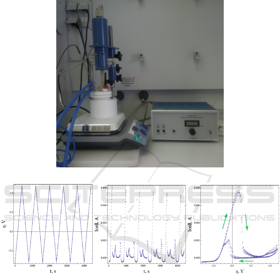
Figure 2: Cyclic voltammetry: experimental setup.

Figure 3: Cyclic voltammetry. From left to right: voltage proﬁle, current proﬁle, current-voltage characteristics with hysteresis

effect.

Fig.3 middle. In coordinates (η, I

cell

) it corresponds

to a closed cycle, shown on Fig.3 right. This curve

in alkaline methanol oxidation experiments demon-

strates a typical hysteresis effect, i.e., the path for in-

creasing voltage does not coincide with the decreas-

ing one. The reasons for this effect and the relation

with other types of measurements will be discussed

below.

Between different measurements, one can also

change concentration of the dissolved reagents c

the temperature T and the period T

. In this way

one has not a single experiment, but a set of exper-

iments which should be simultaneously ﬁt by the ki-

netic model.

Surface coverage proﬁles θ

(t) are generally not

measurable. Although their rough estimation can be

done with the aid of Fourier Transform Infrared Spec-

troscopy (FTIR, (Grifﬁths and de Hasseth, 2007)), the

precision of this approach is not sufﬁcient yet. The

usual way to reconstruct the kinetics is the model

based parameter identiﬁcation.

SIMULTECH 2018 - 8th International Conference on Simulation and Modeling Methodologies, Technologies and Applications

282

4 PARAMETER

IDENTIFICATION

We use Mathematica (Mathematica 11, 2018) for

analysis of cyclovoltagramms. For solution of the

system (4) we use algorithm NDSolve, providing

a generic, stable and robust numerical integrator

of differential equations. The algorithm supports a

bundle of methods, both explicit (ExplicitEuler,

ExplicitRungeKutta, ExplicitMidpoint) and

implicit (Adams, BDF, ImplicitRungeKutta,

SymplecticPartitionedRungeKutta) ones. Ex-

plicit methods require less computational effort per

step, but perform more steps to ensure stability.

Implicit methods can go in large steps, but each step

is computationally expensive. Generally, for stiff sys-

tems implicit methods are preferred. The algorithm

estimates the stiffness of the system, based on the

dominant eigenvalue of the Jacobian. Dependently

on this estimation and theoretically known stability

regions of the integration methods the algorithm

selects a suitable method in respect both to the

stability and precision criteria. Precision of the

integration is internally estimated by Richardson’s

formula: e = |y

− y

|/(2

− 1), where p is the order

of the integration method, |y

− y

| is a difference of

integration results, performed with a single step h and

two sequential half-steps h/2. The step is automati-

cally adapted to keep the error estimator just within

the absolute and relative tolerance bounds, speciﬁed

by parameters AccuracyGoal and PrecisionGoal.

One more convenient feature of NDSolve is a pos-

sibility to solve both Cauchy initial value problems

and boundary problems. We are mainly interested

in periodical solutions of the system (4), which can

be found by setting linear boundary conditions of the

type x(T

) = x(0). The considered system possesses a

polynomial right hand side with periodic coefﬁcients,

due to explicit periodical dependence η(t), entering

in some coefﬁcients. In our numerical experiments,

the system rapidly, in one-two periods, converges to

a limiting cycle, corresponding to the periodical so-

lution. Therefore, an alternative method is to solve

Cauchy initial value problem with an arbitrary start-

ing point, e.g., free electrode θ

= 1, and wait some

periods till convergence.

For the parameter identiﬁcation several capabili-

ties of Mathematica can be used.

Interactive Parameter Study can be performed with

a tool Manipulate. It allows to attach interactive ma-

nipulators (sliders) to the model parameters, while the

results are presented as a collection of plots. The sys-

tem is reevaluated and the results are replotted ev-

ery time when the value controlled by the manipu-

lator is changed. Fig.4 shows an example of usage

of the interactive manipulators for parameter study in

cyclic voltammetry of alkaline methanol oxidation.

The manipulators on the left represent reaction co-

efﬁcients, varied in logarithmic scale in user speci-

ﬁed limits. Each manipulator can be opened, reveal-

ing additional ﬁeld with numerical value and a set of

buttons for animation and stepwise increments. The

current set of parameters is permanently available for

the user in a form of a list and can be printed out,

exported, etc. with standard commands. The central

plot shows a cyclovoltagramm, modeled (red line) vs

measured (blue points). The right plot shows a pe-

riod of evolution for θ values. The ordinal number

of reagent is encoded by a color scheme: red, green,

blue, cyan, magenta, brown for 1-6 and black for 0,

free electrode. The latency of the tool is 0.5 – 1.5

seconds (on 3 GHz CPU), dependently on the number

of cyclovoltagramms to evaluate and plots to display.

It provides the interactive performance, necessary for

parameter study. The tool allows to explore solution

space, immediately observing the inﬂuence of the pa-

rameters, various features and effects in the results

(peaks, dips, shifts, etc.) and compare the modeled

results with measured data.

Automatic Global Optimization can be done with

the algorithm NMinimize. It aggregates a collec-

tion of derivative free methods, attempting to ﬁnd a

global minimum of a given objective function in a

domain, speciﬁed by a set of equality and inequality

constraints. It is commonly known, that global op-

timization is a computationally hard task, especially

for non-linear multidimensional problems. An addi-

tional difﬁculty in our case is that optimization param-

eters, reaction constants, in logarithmic scale do not

have a priori speciﬁed limits. Exponential terms in

the equations can change their contribution by dozens

of orders, also the constants are multiplied by cover-

age values, which in molecular chemistry can be ar-

bitrary small and still provide considerable effects. It

is clear, that in the given problem global optimization

by any method becomes a game of chance. A default

strategy of NMinimize is ﬁrst to apply NelderMead

“downhill simplex” method, and, in the case of poor

performance, switch to DifferentialEvolution,

which is similar to genetic algorithm, and adapted

to real number optimization. Alternatively, the user

can switch to RandomSearch, a multiply restarted lo-

cal optimizer, for which the user can select between

PenaltyFunction and InteriorPoint constraint

minimizers. As a last resort, SimulatedAnnealing

can be used, which emulates a physical process of

a melted metal cooling, asymptotically reaching the

globally minimal energy state. For this purpose, an

Parameter Identiﬁcation in Cyclic Voltammetry of Alkaline Methanol Oxidation

283

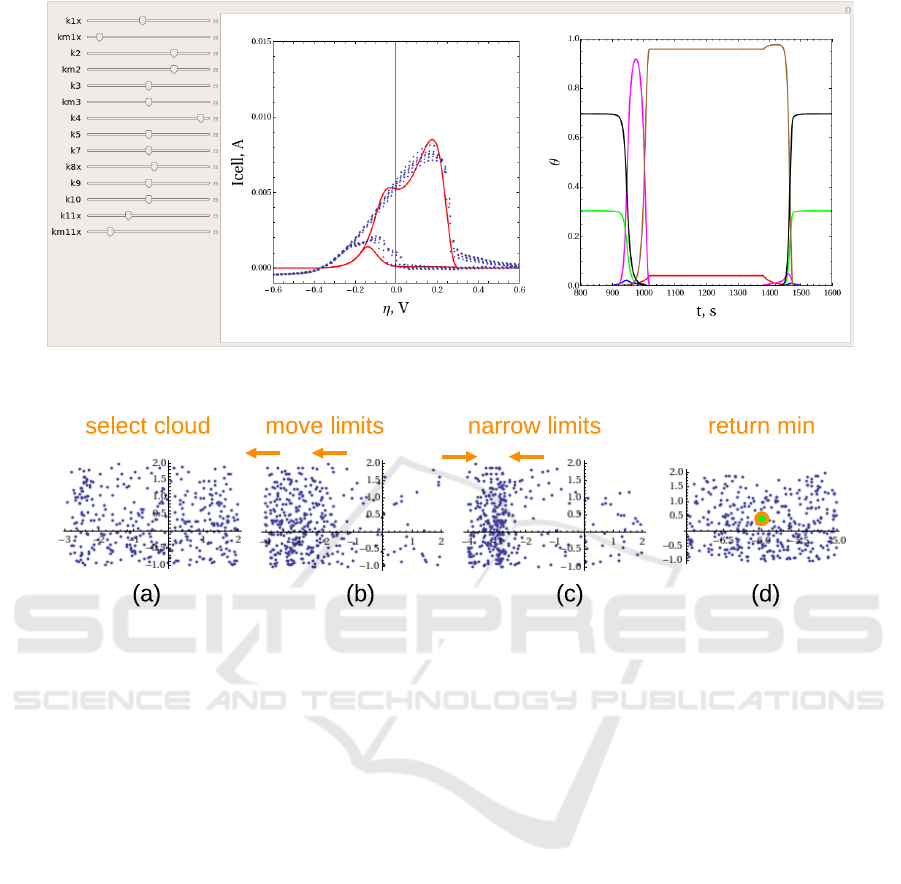
Figure 4: A tool for interactive parameter study. On the left – sliders for variation of parameters, in the center – CV plot,

on the right – surface coverage proﬁles.

Figure 5: Illustration of Iterative Monte Carlo algorithm.

extremely slow cooling schedule must be used: T ∼

1/logt, here t is time, T is the absolute temperature.

While global optimization methods are consid-

ered, also deep local minima are of interest, not

only a single global minimum. In our application,

NMinimize with default settings requires 5000 itera-

tions and 35 min (on 3 GHz CPU) for convergence.

The quality of the minimum is usually comparable

with the other methods. However, in the parameter

identiﬁcation problems with several deep local min-

ima of χ

, all of them may become interesting. Such

local minima can reveal hidden discrete symmetries

of the problem, or, in our case, can indicate several al-

ternative chemical mechanisms, explaining the same

experimental data. Therefore, we have to involve

more exhaustive methods for seaching the alternative

solutions.

Traditional Monte Carlo, also known as Direct

Search method uses a random sampling of parameter

space and an iterative strategy of its reﬁnement. For

example, one can use the following procedure:

Algorithm (Iterative Monte Carlo)

run: generate N random points

in specified limits

select cloud: χ

< threshold

plot cloud in 2D projections (k

)

if cloud is on the border,

move limits,

repeat run

if cloud is localized,

narrow limits,

repeat run

return min over the cloud.

Fig.5 illustrates the work of the algorithm. On the

step (a) the multidimensional cloud χ

< threshold is

selected, here presented in a certain (k

) projection.

The threshold is adjusted to have approximately 500

points in the cloud. The parts (b) and (c) show moving

and narrowing steps. At the end of iterations, at step

(d), the minimum over the cloud is returned.

In our settings, generation of one population of

N = 120000 points requires 6 hours (on 3 GHz CPU),

and one needs 3-5 iterations for convergence. The ad-

vantage of this algorithm is a possibility to branch it-

erative process towards several solutions and an avail-

ability of a large amount of data, representing the be-

havior of χ

in the tested hypervolume. It allows, in

particular, to detect the directions, on which χ

is al-

most independent. These directions represent contin-

SIMULTECH 2018 - 8th International Conference on Simulation and Modeling Methodologies, Technologies and Applications

284

uous symmetries of the system and will be discussed

in details below.

5 RESULTS

Fig.6 shows the results of ﬁtting of experimen-

tal CV plot, measured for concentration of KOH

0.1M, CH

OH 0.5M and temperature 300.75K. Gen-

erally, for randomly selected point in the space of k-

parameters, hysteresis effect is negligible, as shown

on Fig.6 left. Hysteresis effect is present only for a

thin subset of parameters, complicating additionally

the parameter identiﬁcation procedure.

A simple estimation by the order of magnitude

cell

∼ kFA shows that I

cell

∼ 10 mA and FA ∼

1 Cl m

/mol correspond to k ∼ 10

−3

mol/(m

s). The

scale of dynamics τ ∼ C

act

/k ∼ 0.1 s, characterizing a

typical delay in solutions of differential equations, is

much smaller than the period T

= 800 s of CV curve.

So small delay time cannot lead to the visible hys-

teresis, therefore, hysteresis becomes a rare effect in

parametric space and requires special explanations.

Such behavior can appear near the stationary state

with almost degenerate Jacobi matrix. Let eigenval-

ues of Jacobi matrix J be |λ

max

|  |λ

min

|, correspond-

ing to a case of stiff system. Note, that eigenvalues λ

coincide with the poles in EIS measurements (Clees

et al., 2017), while the eigenvectors v are the eigen-

modes of the equation δ

θ = Jδθ, linearizing our sys-

tem in the vicinity of the stationary state, δθ = ve

λt

Note, that λ < 0 by Lyapunov’s stability criterion and

that τ = 1/|λ|. Thus, small λ correspond to large τ,

nearly degenerate systems possess large delay time.

This gives an explanation not only for anomalously

large hysteresis in CV, but also for slow relaxation

to the stationary state in PC analysis and for strong

hierarchy in EIS spectra, mentioned in (Clees et al.,

2017). In Appendix we give an analytical estimation

of the hysteresis effect in linear approximation, show-

ing that the degenerate Jacobian indeed leads to the

large hysteresis.

A particular mechanism for origination of the stiff

system can be a presence of a reagent, weakly coupled

to the rest of reactions, i.e., all reactions involving this

reagent have small reaction constants. Although this

reagent is weakly coupled, it can occupy free surface

of the electrode and inﬂuence the dynamics through

-variable, in this way producing hysteresis effect.

Looking on the reaction graph on Fig. 1, we see that if

this reagent is located in the main chain, such decou-

pling will break the oxidation process. This will pro-

duce the current in the range of microamperes, typical

for experimental measurements with pure KOH with-

out a fuel. To have simultaneously large current and

large hysteresis, the decoupled reagent must be lo-

cated in one of parallel branches of the reaction graph.

Four such places can be identiﬁed, shown by orange

frames on Fig. 1. Correspondingly, our search proce-

dure also ﬁnds four islands of solutions.

Fig.6 center shows the best match results with de-

coupled reagents CO

(red solid line, scenario 1) and

COOH

(green dashed line, scenario 2). Scenario 1

shows similarity with experimental CV shape, how-

ever, it possesses a sharp shoulder with rapid current

variation. This shape is also very sensitive to the vari-

ation of reaction constants. In scenario 2 the optimal

solution possesses less similarity with the experiment.

Fig.6 right shows the best match results with de-

coupled PtO in reactions r

(green dashed line, sce-

nario 3) and r

(red solid line, scenario 4). These

scenarios represent different mechanisms of platinum

oxidation and both have a good match with the ex-

periment. The smoother and better matching shape

corresponds to sequential mechanism in scenario 4.

Table 3 represents the best ﬁt results for all four solu-

tions with their χ

. For reaction constants their loga-

rithms are given:

= log

/[mol/(m

s)]). (7)

Fig.7 shows one more interesting result, found by

the search procedure. It shows the clouds of points

with χ

< threshold in projections to (k

) and

) planes, in logarithmic scale. Straight lines,

visible on these plots show that χ

possesses sta-

ble minimum in perpendicular direction, but shallow

minimum along this line. In other words, the reac-

tion dynamics depends mainly on ratios k

, k

and only those ratios can be stably determined in the

experiment.

6 CONCLUSION

We have presented the methods for parameter identi-

ﬁcation in cyclic voltammetry of alkaline methanol

oxidation. The process involves 11 elementary re-

actions, 9 main reagents and is described by a sys-

tem of 6 non-linear differential equations. For pa-

rameter identiﬁcation we use a combination of auto-

matic global optimization methods, traditional Monte

Carlo and interactive parameter study. Typically, the

integration of the system requires 0.5 sec on 3GHz

CPU. Automatic global optimization requires 5000 it-

erations and 35 min per solution. Monte Carlo gen-

eration of one population of 120000 points requires

6 hours and the related iterative algorithm requires 3-

5 such populations for convergence.

Parameter Identiﬁcation in Cyclic Voltammetry of Alkaline Methanol Oxidation

285

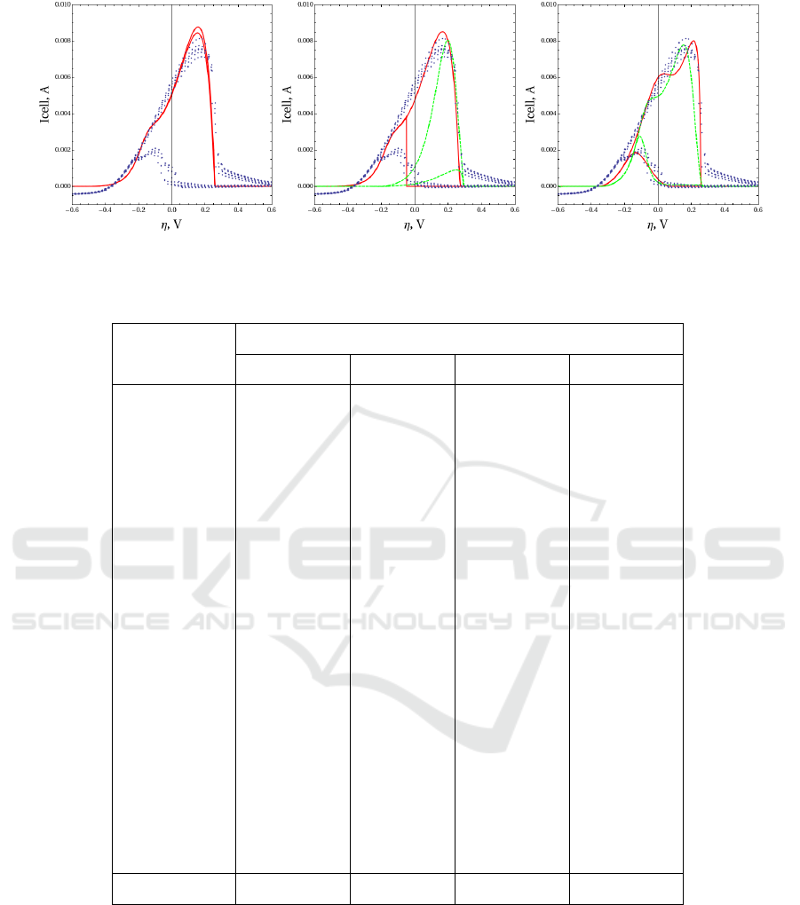
Figure 6: Fitting results. On the left – a typical point with small hysteresis, in the center – optima for scenarios 1 (red solid)

and 2 (green dashed), on the right – optima for scenarios 3 (green dashed) and 4 (red solid).

Table 3: The results of the ﬁt.

Log Constants Scenarios

1 2 3 4

0.00563922 -0.943937 -0.547725 0.0522747

−1

-6.79587 -4.02246 -3.94555 -3.94555

2.15543 1.49158 0.452275 0.752275

−2

2.17691 0.206631 0.512761 0.512761

0.867985 0.669569 4.74111 5.04111

−3

-6.98732 -3.55996 -3.01602 -2.61602

-6.0547 -1.42416 -0.126364 -1.12636

-6.80188 -0.920436 0.128806 0.128806

-0.680335 -2.95533 0.281251 0.281251

-4.45484 -6.6238 -3.64495 -2.64495

-7.0526 -6.47801 1.79963 1.79963

-2.57335 -12.2244 -1.31402 -1.51402

– – -4.04773 –

−11

– – -6.29566 –

– – – -4.84773

−12

– – – -6.09566

/[A

] 0.000170361 0.00102207 0.000332658 0.000161844

As a result of our parameter study, we have found

4 optima corresponding to different mechanisms of

the underlying chemical process. All scenarios intro-

duce a reagent, weakly coupled to the rest of the re-

actions and differ by selection of this reagent. The

weakly coupled reagent has slow kinetics, on the

other hand it occupies free electrode surface and is

able to block the cell current. In this way it pro-

duces the hysteresis effect observable in experimen-

tal plots, being slowly accumulated in the increasing

voltage phase and slowly reduced in the decreasing

one. The weak coupling of the reagent is also respon-

sible for high condition number of the system matrix,

leading to slow convergence of experimental polariza-

tion curves and strong hierarchy of electroimpedance

spectra.

The best match for every scenario is presented and

the details of the related kinetics are discussed.

SIMULTECH 2018 - 8th International Conference on Simulation and Modeling Methodologies, Technologies and Applications

286

Figure 7: Correlation of parameters k

, k

and k

REFERENCES

Bard, A. J. and Faulkner, L. R. (2000). Electrochemical

Methods: Fundamentals and Applications. Wiley.

ack, T. (1996). Evolutionary Algorithms in Theory and

Practice. Oxford University Press, New York.

Beden, B. et al. (1982). Oxidation of methanol on a plat-

inum electrode in alkaline medium: effect of metal

ad-atoms on the electrocatalytic activity. J. Electroan-

alytical Chem., 142:171–190.

Ciucci, F. (2013). Revisiting parameter identiﬁcation in

electrochemical impedance spectroscopy: Weighted

least squares and optimal experimental design. Elec-

trochimica Acta, 87:532–545.

Clees, T. et al. (2014a). Focused ultrasonic therapy plan-

ning: Metamodeling, optimization, visualization. J.

Comp. Sci., 5(6):891–897.

Clees, T. et al. (2014b). Quasi-Monte Carlo and RBF Meta-

modeling for Quantile Estimation in River Bed Mor-

phodynamics. In Obaidat, M. S. et al., editors, Sim-

ulation and Modeling Methodologies, Technologies

and Applications, Advances in Intelligent Systems and

Computing 319, pages 211–222. Springer.

Clees, T. et al. (2017). Electrochemical Impedance Spec-

troscopy of Alkaline Methanol Oxidation. In Proc.

INFOCOMP 2017, The Seventh International Confer-

ence on Advanced Communications and Computation,

pages 46–51. IARIA.

Gamry Instruments (2018). Basics of Elec-

trochemical Impedance Spectroscopy.

http://www.gamry.com/application-notes/EIS/basics-

of-electrochemical-impedance-spectroscopy. Online

tutorial.

Grifﬁths, P. and de Hasseth, J. A. (2007). Fourier Transform

Infrared Spectrometry. Wiley-Blackwell.

Ilonen, J. et al. (2003). Differential Evolution Training Al-

gorithm for Feed Forward Neural Networks. Neural

Proc. Lett., 17:93–105.

Krewer, U. et al. (2006). Impedance spectroscopic analy-

sis of the electrochemical methanol oxidation kinetics.

Journal of Electroanalytical Chemistry, 589:148–159.

Krewer, U. et al. (2011). Electrochemical oxidation of

carbon-containing fuels and their dynamics in low-

temperature fuel cells. ChemPhysChem, 12:2518–

2544.

Mathematica 11 (2018). Reference Manual.

http://reference.wolfram.com.

Nikitin, I. et al. (2012). Stochastic analysis and nonlinear

metamodeling of crash test simulations and their ap-

plication in automotive design. In Browning, J. E.,

editor, Computational engineering: design, develop-

ment, and applications, pages 51–74. Nova Science.

Otten, R. H. J. M. and van Ginneken, L. P. P. P. (1989). The

Annealing Algorithm. Kluwer.

Press, W. H. et al. (1992). Numerical Recipes in C: Chap.

15. Cambridge University Press.

Strutz, T. (2016). Data Fitting and Uncertainty: A practi-

cal introduction to weighted least squares and beyond.

Springer.

achter, A. and Biegler, L. T. (2006). On the implemen-

tation of an interior-point ﬁlter line-search algorithm

for large-scale nonlinear programming. Mathematical

Programming, 106:25–57.

APPENDIX: LINEAR ESTIMATION

OF HYSTERESIS EFFECT

Consider a system of differential equations:

act

= f (θ,η) (8)

in the limit C

act

→ 0. In this way we emulate the sys-

tems with small delay time τ = C

act

/k → 0.

The solution is located in the vicinity of the sta-

tionary curve

f (θ

∗

,η) = 0, (9)

where both θ

∗

and η depend on t. After differentia-

tion, we have

Jθ

∗

∂ f

∂η

= 0, J =

∂ f

∂θ

. (10)

Further, in linearized equations

act

(θ

∗

+ δθ

) = f (θ

∗

,η) +Jδθ, (11)

omitting small δθ

term and using (9) and (10), we

have

δθ = −C

act

−2

∂ f

∂η

. (12)

Substituting it to the linearized expression for current,

we obtain

δI =



∂I

∂θ



δθ = (13)

−C

act



∂I

∂θ



−2



∂ f

∂η



Parameter Identiﬁcation in Cyclic Voltammetry of Alkaline Methanol Oxidation

287

As a result, we see, that a deviation of current from the

stationary curve changes sign with η

, i.e., possesses

the hysteresis effect. In general position, the vectors

on the left and on the right of J

−2

in (13) do not co-

incide with annulators of Jacobian, i.e., its left and

right eigenvectors with tending to zero eigenvalue. In

this case, the amplitude of hysteresis effect tends to

inﬁnity, in the limit when the Jacobian becomes de-

generate:

detJ → 0, δI → ∞. (14)

This condition can be used only as an indicator of

hysteresis effect. With increasing δI, one will need

to apply the next order corrections to approximate its

value.

SIMULTECH 2018 - 8th International Conference on Simulation and Modeling Methodologies, Technologies and Applications

288