
Autonomous Trail Following using a Pre-trained Deep Neural Network
Masoud Hoveidar-Sefid and Michael Jenkin
Electrical Engineering and Computer Science Department and York Centre for Field Robotics,
Lassonde School of Engineering, York University, Toronto, Canada
Keywords:
Autonomous Navigation, Trail Following, Path Finding, Deep Neural Networks.
Abstract:
Trails are unstructured and typically lack standard markers that characterize roadways; nevertheless, trails
can provide an effective set of pathways for off-road navigation. Here we approach the problem of trail
following by identifying the deviation of the robot from the heading angle of the trail through the refinement
of a pretrained Inception-V3 (Szegedy et al., 2016a) Convolutional Neural Network (CNN) trained on the
ImageNet dataset (Deng et al., 2009). A differential system is developed that uses a pair of cameras each
providing input to its own CNN directed to the left and the right that estimate the deviation of the robot with
respect to the trail direction. The resulting networks have been successfully tested on over 1 km of different
trail types (asphalt, concrete, dirt and gravel).
1 INTRODUCTION
A key requirement for off-road autonomous naviga-
tion is to be able to follow a certain path or trail in
a natural and unstructured environment. The robot
continuously follows a trail and at each instant takes a
sensor snapshot of the trail “in front” of the robot. The
goal is to take this snapshot and to estimate the devi-
ation of the robot with respect to the direction of the
trail and to then generate an appropriate motion com-
mand that moves the robot along the trail. The road
fallowing version of the problem is aided by many
detectable and well known features associated with
highways and streets. This is to be compared to the
somewhat unstructured nature of trails. The diversity
of trail types presents many challenges for the task of
fully autonomous navigation.
There are many possible approaches to trail fol-
lowing, however, this work utilizes an Inception-
V3 (Szegedy et al., 2016b) CNN pretrained on the
ImageNet dataset (Deng et al., 2009) to estimate trail
deviation. Although the Inception-V3 CNN trained
on ImageNet can be used to recognize trail heading, it
has difficulty in distinguishing between deviations to
the left and the right. In order to overcome this limita-
tion here we propose a differential approach that uses
two cameras, each using the same tuned CNN based
on the Inception-V3 pre-trained network to address
the trail following task.
2 PREVIOUS WORK
There is a large road following literature associ-
ated both with ‘off-road’ roads as well as hard sur-
face roadway following. Space does not permit a
full review of these approaches here, and the inter-
ested reader is directed to (DeSouza and Kak, 2002)
and (Hillel et al., 2014) for surveys of the field.
There are many potential approaches to trail fol-
lowing. Here we concentrate on a CNN-based ap-
proach. The last ten years or so have seen a resur-
gence in NN-based approaches to this problem aided
in part by substantive increases in computational
power that enables ‘deep’ networks to be constructed
and the vast amounts of labeled data that now exists
to train these networks. NN-based approaches to road
or trail following generally fall into one of two basic
categories, systems that classify the state of the robot
relative to the road and then use this information to
steer the vehicle, and approaches that map sensor data
to steering angle directly.
Road Surface Detection. This category of ap-
proaches first segments image pixels into road or non-
road classes. This information is then used to es-
timate the best steering angle to keep the robot on
the road while moving the robot forward. These ap-
proaches treat the problem as a classification prob-
lem (which pixels are road pixels) exploiting the wide
range of classification approaches that are based on
Hoveidar-Sefid, M. and Jenkin, M.
Autonomous Trail Following using a Pre-trained Deep Neural Network.
DOI: 10.5220/0006832301030110
In Proceedings of the 15th International Conference on Informatics in Control, Automation and Robotics (ICINCO 2018) - Volume 1, pages 103-110
ISBN: 978-989-758-321-6
Copyright © 2018 by SCITEPRESS – Science and Technology Publications, Lda. All rights reserved
103

CNN’s. For example, (Mohan, 2014), presents a
deep deconvolutional network architecture that incor-
porates spatial information around each pixel in the
labeling process. (Brust et al., 2015) and (Mendes
et al., 2016) use small image patches from each frame
in order to label the center pixel of each patch as ei-
ther road or non-road. These patches are fed into a
trained CNN to classify the label of the center pixel
of that patch. These algorithms use spatial infor-
mation associated with each pixel in order to label
that pixel with high confidence. (Oliveira et al., 2016)
present a method for road segmentation with the aim
of reaching a better trade-off between accuracy and
speed. They introduce a CNN with deep deconvolu-
tional layers that improves the performance of the net-
work. Another advantage of this method is that it uses
the entire image as an input; not different patches of
each frame and this helps to make the algorithm run
faster and be more efficient.
Steering the Robot Directly. Work here can be
traced back to the late 1980’s and works such as
ALVINN (Pomerleau, 1989). This approach uses a
set of driver’s actions captured on different roads such
as one lane, multi-lane paved roads and also unpaved
off-roads, to train the neural network architecture of
the robot to return a suitable steering command to the
robot. Work following this basic strategy continues
today. To take but one recent example, NVIDIA (Bo-
jarski et al., 2016) designed a system to train a CNN
on camera frames with respect to the given steering
angle of a human driver for each frame. An instru-
mented car is outfitted with a camera that simulates
the human driver’s view of the road, and a human
drives the vehicle while the camera input and human
steering commands are collected. A CNN is then con-
structed from this dataset using the human steering
angle as ground truth.
CNN’s have also been used to drive a robot on
off-road trails and one such approach is presented
in (Giusti et al., 2016). This work uses a machine
learning approach for following a forest trail. Rather
than directly mapping image to steering angle this
approach categorizes the input image into one of
’straight’, ’left’ or ’right’ and then uses the distribu-
tion of likelihoods over these three categories to com-
pute both a steering angle as well as an appropriate
vehicle speed. In order to collect training data three
cameras are mounted on the hip of a hiker, one point-
ing ’forward’ and one yawed to the right and the other
one yawed to the left. Data is collected while the ’for-
ward’ camera is aligned with the trail. These three
cameras are set up with a 30 degrees yaw from each
other on the head of a hiker to record the dataset.
Table 1: TrailNet dataset training hyperparameters.
Training hyperparameters Value
epochs 5
learning rate 0.02
train batch size 100
validation batch size 100
random brightness ±15%
# images per label for training 5000
# images per label for validation 625
# images per label for testing 625
Their dataset consists of 8 hours of video in forest-
like trails and images are captured in a way that the
hiker always looks towards the direction of the trail.
Therefore, in a classification task, the central cam-
era is labeled as “go straight”, the left camera is la-
beled as “turn right” and the right camera is labeled
as “turn left”. These labels are then used to train a
CNN in order to perform the classification task and
outputs a probability of each class as a softmax func-
tion. They used a 9 layer neural network in order
to do the classification task. These layers consist of
4 back to back convolutional and max-pooling lay-
ers followed by a 2,000 neuron fully connected layer
and finally a classification layer (output layer) with
three neurons which returns the probability of occur-
rence of each label. This DNN is based on the archi-
tecture used in (Ciregan et al., 2012). For evaluation
purposes, the accuracy of this classifier is calculated
based on the maximum probability of softmax func-
tion in the output of DNN. The reported accuracy is
85.2% for the classification task between three labels
of “go straight”, “turn right” and “turn left”.
3 TrailNet DATASET
Key to a CNN-based approach is an appropriate
dataset to train the network. For this work we col-
lected the TrailNet dataset of different trails under
various trail and imaging conditions (its capture is
inspired by the approach presented in (Giusti et al.,
2016)). TrailNet
1
consists of images captured from
wide field of view cameras of different trail types,
where each class of images has a certain deviation an-
gle from the heading direction of the trail. In order to
study the effect of surface type of the trails, each of
the TrailNet dataset are further divided by trail types:
(1) asphalt, (2) concrete (3) dirt and (4) gravel. Trail-
Net was captured with three omnidirectional cameras.
1
TrailNet is available for public use at http://vgr.lab.
yorku.ca/tools/trailnet
ICINCO 2018 - 15th International Conference on Informatics in Control, Automation and Robotics
104

Table 2: Detailed test accuracy results of the straight/not-straight method with the three narrow camera geometry setup on all
trail types. The 0
◦
and overall columns show recognition rate for the two classes. Performance is also broken down for each
of the −60
◦
and +60
◦
categories separately.
Test accuracy Subcategories accuracy
Training dataset Overall Not-straight Straight +60
◦
−60
◦
0
◦
Asphalt 99.90% 99.95% 99.90% 100.0% 99.90% 99.90%
Concrete 99.75% 100% 99.20% 100.0% 100.0% 99.20%
Dirt 97.77% 100% 99.20% 100.0% 100.0% 99.30%
Gravel 99.13% 99.88% 98.14% 100.0% 99.24% 98.14%
Each of the cameras is a Kodak Pixpro SP360 (kodak,
2016), which provides a fish eye camera with a 214
◦
degree of vertical field of view at 30 frames per sec-
ond with a resolution of 1072 × 1072 pixels. A Pi-
oneer 3-AT robot (p3at, 2017) was used as a mobile
base in this work. During training the three cameras
were mounted on a detachable circular mount on top
of the robot, while during trail following only the two
cameras directed to the left and right were used.
4 FINE TUNING A PRETRAINED
CNN MODEL
Transferring knowledge from a trained network on a
given task to another network operating on a target
task is called transfer learning and a survey of dif-
ferent approaches in this domain is presented in (Pan
and Yang, 2010). The basic approach involves taking
a pre-learned CNN and then surrounding this CNN
with a small number of layers and then training just
these layers on the specific problem. In this approach
the last layer of the network (also known as classifi-
cation layer) which is a fully connected layer, is re-
placed with two new fully connected layers and only
the parameters of these two layers are trained on the
new dataset. This fine tuning approach transfers the
mid-range features learned by the source network and
exploits them in a new classification task. Obtain-
ing a rich and vast annotated dataset on a new task is
a very tedious and sometimes very expensive proce-
dure. As a consequence, the fine tuning approach can
be very helpful when the target task does not have a
huge dataset from which to train a CNN from scratch.
Here we explore using the pre-trained Inception
network to differentiate between straight ahead trails
and trails that are bending away from the straight
ahead direction. In this method, labels are either
straight (i.e., 0
◦
) or not straight (i.e., −60
◦
or +60
◦
).
Hyperparameters used in the following training steps
were common over the different training regimes fol-
lowed and are provided in Table 1. Table 2 shows the
performance on each trail type by their corresponding
trained network.
In order to study the effect of the trail type in the
task of deviation angle recognition on trails, the per-
formance of each road-type (asphalt, concrete, dirt,
gravel) network was tested on a test set from each of
the trail types. Table 3 shows the performance con-
fusion matrix. The “correct” recognizer works well
on the “correct” trail type (the diagonal in Table 3)
while the “wrong” recognizer shows reasonably good
accuracy on the “wrong” trail type with some excep-
tions. The dirt network shows a reasonably good per-
formance on all the other trail types, the asphalt net-
work is reliable for asphalt and concrete, the concrete
network shows a good performance only on concrete,
and the gravel network also has a good ability to rec-
ognize the correct labels for the concrete dataset and
the gravel dataset itself. But for best performance, a
properly tuned trail-specific CNN performs best.
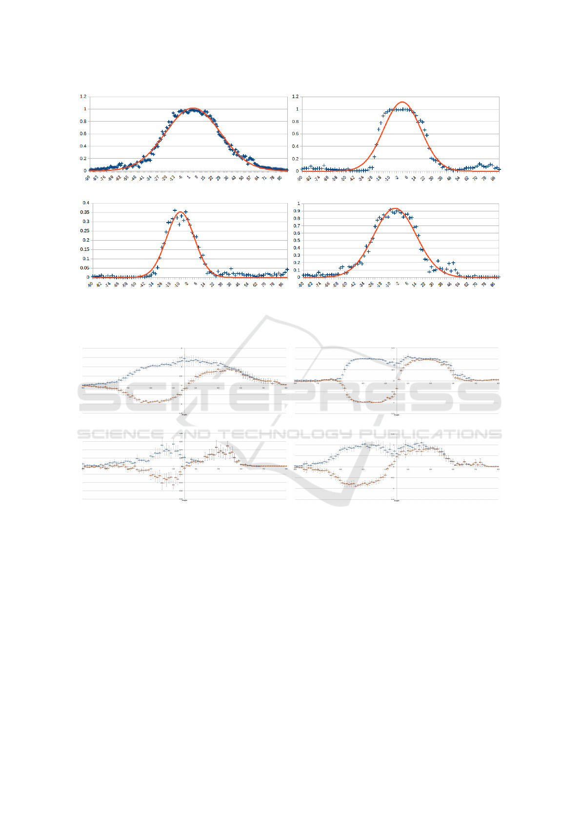
The ability of the fine tuned Inception-V3 CNN’s
to differentiate between straight ahead and not-
straight ahead classes can be used to develop a dif-
ferential strategy for trail following. Figure 1 shows
the 0
◦
classifier output results for each of the classi-
fiers as the roadway curves from −90
◦
to +90
◦
. For
each response curve a normalized Gaussian is fit. The
nature of the fits suggest that the networks have a
symmetrical sensitivity for the positive and negative
deviation angles from the trail. The Gaussian-like re-
sponse fit also suggests that a classical difference of
offset Gaussian (DOOG)(Young et al., 2001)-like ap-
proach could be exploited to combine multiple CNN
response curves to estimate the direction of the trail
relative to the robot.
Table 3: Confusion matrix for the straight versus not-
straight trained networks on the test sets from their cor-
responding trails and other trail types. Poorly performing
network-trail type combinations are highlighted in bold.
Trail type (%)
NN asphalt concrete dirt gravel
asphalt 99.90 96.69 63.78 87.26
concrete 85.34 99.75 66.60 70.10
dirt 92.40 93.95 97.77 95.15
gravel 84.72 98.83 84.33 99.13
Autonomous Trail Following using a Pre-trained Deep Neural Network
105
(a) Asphalt
(b) Concrete
(c) Dirt
(d) Gravel
Figure 1: Blue points in the charts depict the 0
◦
label output results of the trained networks on images between −90
◦
and
+90
◦
on their corresponding trail type. Orange lines show a normalized Gaussian function fitted to the plotted results. The
Gaussian fit is normalized to the maximum of the response curve. Note the different vertical axes for the various plots.
(a) Asphalt CNN (b) Concrete CNN
(c) Dirt CNN
(d) Gravel CNN
Figure 2: Experimental values of G
+
(blue) and G
−
(orange) with standard errors for generic camera geometry but different
CNN terrain types. The horizontal axis of all charts is the angle of the heading of the robot γ with respect to the trail direction.
4.1 Differential Method
Rather than utilizing a single “forward facing” sensor
here we utilize two such sensors each providing input
to their own identical CNN and then utilizes the dif-
ference between two “straight ahead” classifier out-
puts obtained from cameras offset in orientation to the
left and right to encode the trail direction. In order to
find the optimal offset angle between the cameras the
sensitivity functions of the CNN’s with respect to the
deviation angle of the robot γ relative to the trail is
estimated (see Table 4).
Assume that the sensitivity function of the right
and left CNN’s are well described by the Gaussian
distributions are G
1
and G
2
, where G
1
and G
2
have
the same standard deviation σ and means of µ
1
= θ/2
and µ
2
= −θ/2, respectively. The combined sensi-
tivity function of the two CNN’s is computed as the
addition of G
1
and G
2
as G
+
= G
1
+ G
2
. The differ-
ence between G
1
and G
2
is denoted as G
−
= G
1
−G
2
.
In order to have a stable overall sensitivity function
G
+
and preventing G
+
from having a ripple in the
center, θ should be chosen in a way that at γ = 0,
G
1
= G
2
≥ 0.5.
Table 4 shows the characteristics of the Gaussian
distributions of all of the networks on their corre-
ICINCO 2018 - 15th International Conference on Informatics in Control, Automation and Robotics
106
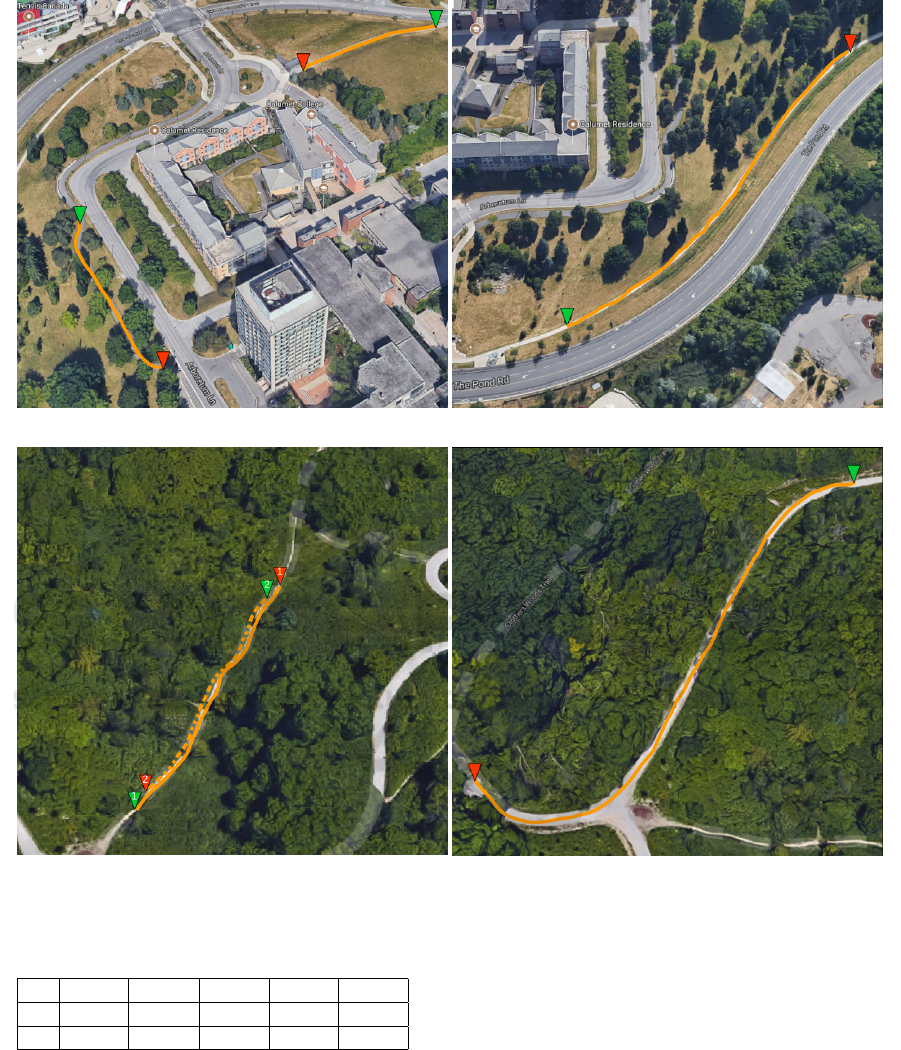
(a) Asphalt map
(b) Concrete map
(c) Dirt map
(d) Gravel map
Figure 3: Overhead views of the test environments.
Table 4: Gaussian model parameters for each network.
NN Asphalt Concrete Dirt Gravel Average
µ 3.96 1.47 -8.86 -5.68 -2.27
σ 24.85 16.99 12.85 19.69 18.59
sponding trail type and their averages across the dif-
ferent trail types. The average standard deviation
σ
avr
= 18.59 was used to establish a generic camera
separation. Figure 2 shows the performance of the
differential CNN’s on the different trail types. G
−
encodes the deviation of the robot from the straight
ahead direction while G
+
encodes the confidence of
this output.
From Trail Orientation to Steering Angle. There
are a number of practical issues involved in comput-
ing a steering command from the estimated trail ori-
entation. First, if the detector cannot detect a road,
then some default steering angle should be chosen or
in a full application this information should also be
sent to higher level control. Second, there is a de-
sire to not oversteer (an overshoot) the vehicle mo-
tion, and finally, if the steering angle is only changing
by a very small amount the robot should not introduce
small zero-mean fluctuations into the steering angle
(the controller should have a deadband region). Prop-
erly addressing all of these issues is beyond the scope
Autonomous Trail Following using a Pre-trained Deep Neural Network
107
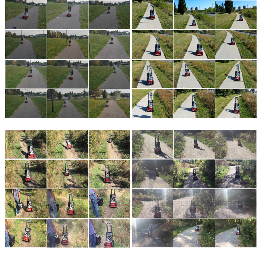
(a) Asphalt
(b) Concrete
(c) Dirt
(d) Gravel
Figure 4: Snapshots taken along the trails.
of this paper, so here we adopt a very simple strategy
for obtaining a steering angle change from the (G+,
G-) pair. If |G
−
| < th
−
, then we assume that the robot
is in a deadband region, and set the change in steering
angle to be zero. If |G + | < th
+
, then the detector
does not detect a trail, and again we set the change in
steering angle to be zero. For other angles we clamp
the output change in steering angle to ±0.1 rad/s. In
all of the operating states of the robot, for the exper-
iments described in the following section, the robot
has a constant forward velocity of 20cm/s.
5 EXPERIMENTAL RESULTS
In order to test the performance of the algorithm for
the task of autonomous driving on trails, field tri-
als were conducted on a range of trail types. Due
to the battery capacities of the robot and the hard-
ware used in this experiments, tests were broken down
into 10 distances of 20 meters long. The following
evaluations were used based on criteria typically used
for autonomous driving systems (see (Bojarski et al.,
2016));
• The maximum distance traveled over the the 20
ICINCO 2018 - 15th International Conference on Informatics in Control, Automation and Robotics
108
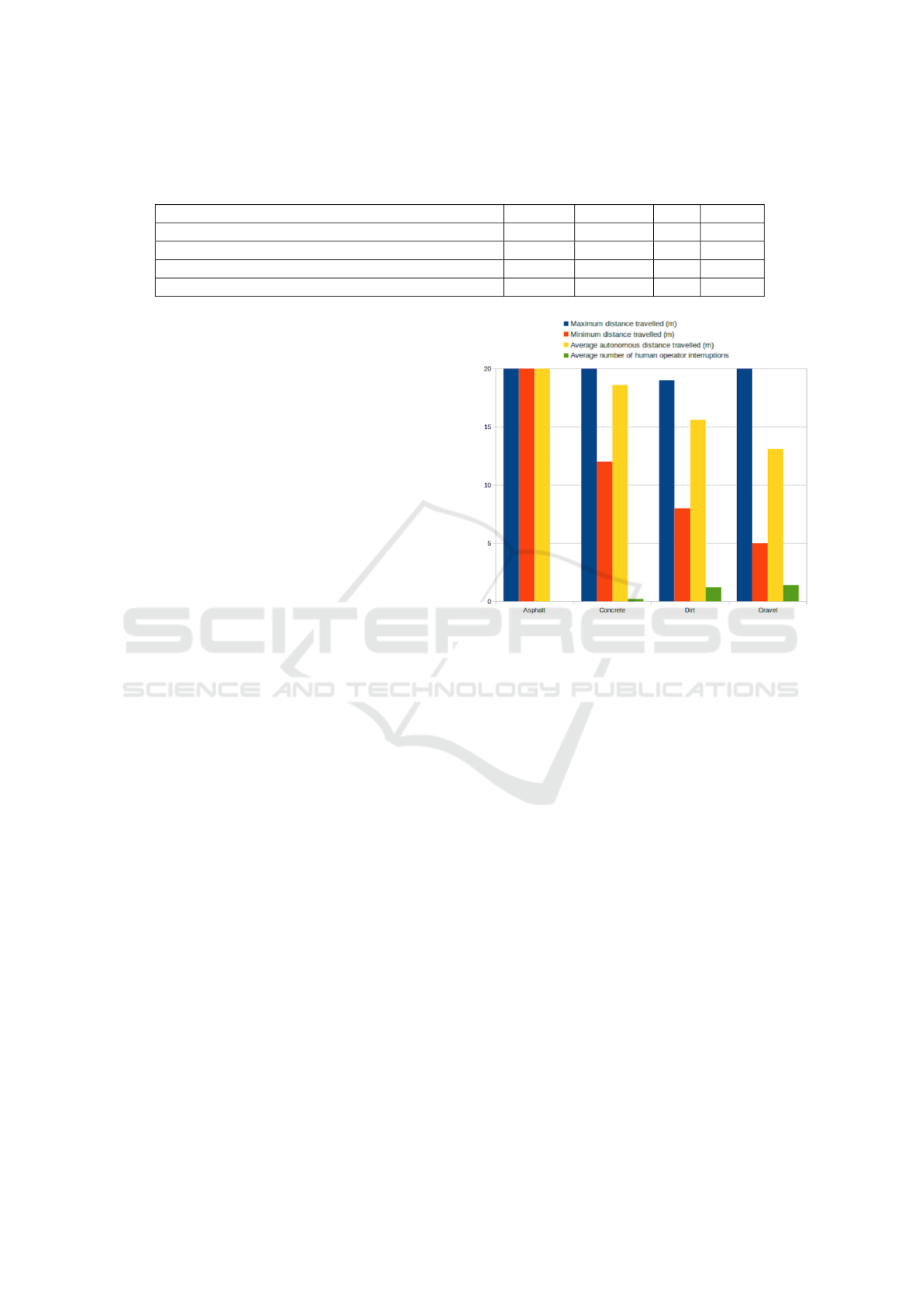
Table 5: Autonomous field trial results for different trail types on 200 meters of paths shown in Figure 3 (a)-(d). The average
values are computed based on the performance of the algorithm over ten different 20 meters pieces of path. Performance of
the algorithm on asphalt and concrete paths was quit good, but deteriorated on dirt and gravel trails.
Parameters Asphalt Concrete Dirt Gravel
Maximum distance travelled (m) 20 20 19 20
Minimum distance travelled (m) 20 12 8 5
Average autonomous distance travelled (m) 20 18.6 15.6 13.1
Average number of human operator interruptions 0 0.2 1.2 1.4
meter test ranges before human intervention was
required.
• The minimum autonomous distance traveled over
each of the ten 20 meter test ranges before human
intervention was required.
• The average autonomous distance traveled over
each of the ten 20 meter test ranges before human
intervention was required.
• The average number of human operator interrup-
tions required in order to drive the vehicle 20 me-
ters.
Figure 3 shows the paths chosen for the test on a map
and Figure 4 provides a film strip of the robot in oper-
ation on all trail types. A chart of the results of the test
on four different trails is shown in Table 5. Figure 5
plots a summary of these results.
The tests showed a number of interesting aspects
of the algorithm. First, the algorithm performed very
well on asphalt and concrete paths with the robot op-
erating perfectly on asphalt and performing on aver-
age over 18m (in a 20m trial) without failure on con-
crete trails. Performance on dirt and gravel trails was
less successful, but still showed quite good perfor-
mance. It is interesting to note that the dirt trail was
much narrower than the other trails tested (see Fig-
ure 5) but that even here performance was quite good.
Worst performance was found on the gravel trail. One
possibility here is that the control algorithm devel-
oped for gravel trails might need to be more tightly
tuned for the gravel as the robot’s tires exhibited poor
performance on this surface.
6 CONCLUSION
This paper presented a refinement learning-based ap-
proach with the use of Inception-V3 network for off-
road autonomous trail following. Experiments eval-
uated the nature, geometry and number of cameras
that might be applied to the problem. Using a DOOG
model a trail following algorithm was successful in
navigating different trail types using a common cam-
era geometry and using tuned CNN’s for different trail
Figure 5: Autonomous test results plot on different trail
types (see Table 5 for details). Vertical axis is in meters for
distance traveled and count for average number of human
operator interruptions.
types. End-to-end testing of the algorithm showed
very good performance on asphalt and concrete paths,
with poorer performance on dirt and gravel. Perfor-
mance on dirt was still quite impressive given the nar-
row nature of such paths.
ACKNOWLEDGMENTS
The support of NSERC Canada and the NSERC
Canadian Field Robotics Network (NCFRN) are
gratefully acknowledged.
REFERENCES
Bojarski, M., Del Testa, D., Dworakowski, D., Firner, B.,
Flepp, B., Goyal, P., Jackel, L. D., Monfort, M.,
Muller, U., Zhang, J., Zhang, X., Zhao, J., and Zieba,
K. (2016). End to end learning for self-driving cars.
arXiv:1604.07316.
Brust, C.-A., Sickert, S., Simon, M., Rodner, E., and Den-
zler, J. (2015). Convolutional patch networks with
Autonomous Trail Following using a Pre-trained Deep Neural Network
109

spatial prior for road detection and urban scene un-
derstanding. arXiv preprint arXiv:1502.06344.
Ciregan, D., Meier, U., and Schmidhuber, J. (2012). Multi-
column deep neural networks for image classification.
In Proc. IEEE CVPR, pages 3642–3649, Providence,
RI.
Deng, J., Dong, W., Socher, R., Li, L.-J., Li, K., and Fei-
Fei, L. (2009). Imagenet: A large-scale hierarchical
image database. In Proceedings of the IEEE Inter-
national Conference on Computer Vision and Pattern
Recognition (CVPR), pages 248–255, Miami, FL.
DeSouza, G. N. and Kak, A. C. (2002). Vision for mobile
robot navigation: A survey. IEEE PAMI, 24(2):237–
267.
Giusti, A., Guzzi, J., Cires¸an, D. C., He, F.-L., Rodr
´
ıguez,
J. P., Fontana, F., Faessler, M., Forster, C., Schmidhu-
ber, J., Di Caro, G., et al. (2016). A machine learning
approach to visual perception of forest trails for mo-
bile robots. IEEE Robotics and Automation Letters,
1(2):661–667.
Hillel, A. B., Lerner, R., Levi, D., and Raz, G. (2014). Re-
cent progress in road and lane detection: a survey. Ma-
chine Vision and Applications, 25(3):727–745.
kodak (2016). The Kodak camera website.
Mendes, C. C. T., Fr
´
emont, V., and Wolf, D. F. (2016). Ex-
ploiting fully convolutional neural networks for fast
road detection. In Proc.IEEE ICRA, pages 3174–
3179, Stockholm, Sweden.
Mohan, R. (2014). Deep deconvolutional networks for
scene parsing. arXiv preprint arXiv:1411.4101.
Oliveira, G. L., Burgard, W., and Brox, T. (2016). Efficient
deep models for monocular road segmentation. In
Proc. IEEE IROS, pages 4885–4891, Daejeon, South
Korea.
p3at (2017). The Pioneer 3-at robot website.
Pan, S. J. and Yang, Q. (2010). A survey on transfer learn-
ing. IEEE Transactions on Knowledge and Data En-
gineering, 22(10):1345–1359.
Pomerleau, D. A. (1989). ALVINN, an autonomous
land vehicle in a neural network. Technical report,
Carnegie Mellon University, Computer Science De-
partment, Pittsburgh, PA.
Szegedy, C., Vanhoucke, V., Ioffe, S., Shlens, J., and Wo-
jna, Z. (2016a). Rethinking the inception architecture
for computer vision. In Proceedings of the IEEE Con-
ference on Computer Vision and Pattern Recognition
(CVPR), pages 2818–2826, Las Vegas, NV.
Szegedy, C., Vanhoucke, V., Ioffe, S., Shlens, J., and Wojna,
Z. (2016b). Rethinking the inception architecture for
computer vision. In Proc. IEEE CVPR, pages 2818–
2826.
Young, R. A., Lesperance, R. M., and Meyer, W. W. (2001).
The gaussian derivative model for spatial-temporal vi-
sion: I. cortical model. Spatial Vision, 14(3):261–319.
ICINCO 2018 - 15th International Conference on Informatics in Control, Automation and Robotics
110
