Can Artiﬁcial Potentials Suit for Collision Avoidance in Factory Floor?

A Case Study of Harmonic Machine-machine Coexistence

Josias G. Batista

, Jos

e L. N. da Silva

and George A. P. Th

Instituto Federal de Educac¸

ao Tecnol

ogica do Cear

a, av. 13 de Maio 2081, Fortaleza, Brazil

Department of Teleinformatics Engineering, Federal University of Ceara, Fortaleza, Brazil

Keywords:

Path Planning, Machine-machine Interaction, SCARA Manipulator.

Abstract:

Despite the existence of well-known approaches for collision prevention in the robotics literature, in present

days the use of manipulators in fabrication processes still relies on safe-zone delimitations, which ultimately

limits automation ﬂexibility. In the present work, we consider going over that paradigm by discussing what if

mobile agents of the fabrication process, i.e., robots could share the same space. In doing that study, the very

classical approach based on artiﬁcial potentials for collision prevention are preferred over modern choices. On

the basis of a hypothetical pick-&-place task experiment, results revealed efﬁcient accomplishment in some of

the considered scenarios.

1 INTRODUCTION

In modern production processes the deployment of ro-

bots in semi- or fully-automatized taks assumed an

important and strategic role for industry; recent re-

ports from the International Federation of Robotics

estimate something over 250 thousands new units of

industrial robots worldwide only in 2015 (IFR, 2017).

Typically, industrial robots operate inside proper cells

in classiﬁed areas designed to provide adequate sepa-

ration between men and machines; it is also recom-

mended the use of sensors for human-presence de-

tection as well as switching-off mechanism in case

of cell invasion by persons. It is to be stressed the

economical consequence of it, since interrupting the

process may cause delays and bring additional pro-

duction costs.

From the point-of-view of increasing ﬂexibility le-

vel of automation, it would be good thing if those

strict recommendations for robot cells could be revi-

sited and production machines and other agents were

let free to share the factory ﬂoor aided by techni-

ques for preventing collisions and process interrupti-

ons as well. This issue may be regarded as a machine-

machine coexistence problem and it is a challenging

one if no previous information about dimension and

shape of the agents is given as well as the agents are

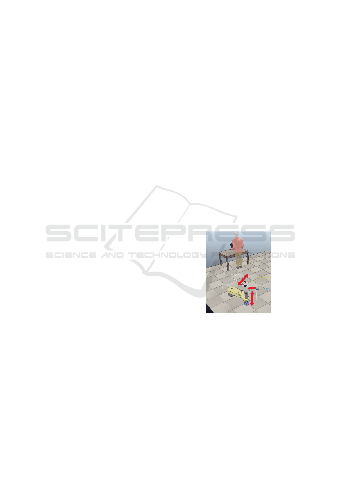
allowed to move arbitrarily in that space, as illustra-

ted in Figure 1. To cover with the need for a non-stop

production, an intelligent robot-assisted automation

system should therefore conjugate real-time obstacle

detection and collision avoidance algorithms.

Figure 1: Various robots sharing workspace.

In the literature, the paradigm of machine-

machine interaction is usually presented as coopera-

tive robotics, in which agents has a common task to

accomplish (Habib, 2014) or, in the context of as-

sistive robotics, in which robots interact to anticipate

human actions thus offering them some kind of assis-

tance like, for instance, in helping at opening a door,

taking up objects, etc (Koppula and Saxena, 2016).

Also interesting is the context of competitive robotics,

in which machines interact as opponents (Pinto et al.,

2016) or more simply in situations of conﬂicting inte-

rests (e.g., those of workspace superposition) (Gayle

et al., 2007).

Batista, J., Silva, J. and Thé, G.

Can Artiﬁcial Potentials Suit for Collision Avoidance in Factory Floor? - A Case Study of Harmonic Machine-machine Coexistence.

DOI: 10.5220/0006832405470556

In Proceedings of the 15th International Conference on Informatics in Control, Automation and Robotics (ICINCO 2018) - Volume 2, pages 547-556

ISBN: 978-989-758-321-6

547

Right in this context the present research is fo-

cused: it brings to light a hypothetical automatized

production process in which mobile robots and ma-

nipulators are the agents having conﬂicting tasks by

discussing how the machine-machine interaction can

be driven towards more efﬁcient and productive pro-

cess (Moellmann et al., 2006). The scenario consi-

dered here is the one illustrated in Figure 1: two au-

tomatic machines with overlapping workspaces share

a given region of the factory ﬂoor and have to deal

with the possibility of iminent collision; the mani-

pulator is doing a pick-and-place task, whereas the

wheel-drive robot is on some transport task in non-

constrained route. The more collisions occur, clearly

the more the robots will limit the efﬁciency of the pro-

ductive process they are engaged in, because the ti-

ming and productivity metrics for performance evalu-

ation will suffer from non-scheduled stops. Collisions

are therefore to be avoided undoubtedly; nothing new.

What is not known in advance and appears as open is-

sue in this hypothetical experiment is the amount of

inﬂuence the chosen strategy for collision avoidance

may have on the on-going production. First of all,

are the classical approaches for collision avoidance of

robots viable for real-time navigation in the conside-

red emulated production scenario? If so, under which

assumptions and operating (or even modelling) con-

straints? Then, how can we quantify the inﬂuence the

chosen collision prevention strategy has on the task

assigned to the robot? Is there any measure from the

scientiﬁc community to be used as indicator of the just

mentioned quantity? Any opportunity for new mea-

sure or even a ﬁgure-of-merit?

Purpose of this paper is to address these questi-

ons through the use of classical approaches in robotics

and traditional concepts from production engineering.

On one side, concerning the strategy for collision pre-

vention, in this study artiﬁcial potential ﬁelds was pre-

ferred over geometric search approach for its simpli-

ﬁcity and popularity as the literature review reveals.

On the other side, to evaluate task accomplishment, it

was adopted an indicator named Overall Equipment

Efﬁciency, which takes into account availability, qua-

lity and performance itself of a given machine.

The remainder of the paper is organized in the fol-

lowing sections: after a literature review about the

employment of artiﬁcial potential ﬁeld methods for

path planning in robotics, section 3 presents the the-

oretical ingredients such as the manipulator kinema-

tics, the adopted Fuzzy controller design, the basics of

artiﬁcial potentials, as well as the metrics used to as-

sess the efﬁciency of the transport task studied here.

Section 4 contains the results and respective discus-

sion, which are followed by conclusions.

2 LITERATURE REVIEW

Artiﬁcial potential ﬁeld (APF) methods are very clas-

sical choice for reactive path planning of robots de-

aling with moving obstacles; originally proposed in

(Khatib, 1986) for collision avoidance of manipula-

tors and mobile robots as well, it is still very popular

because it is fast, simple and mathematically elegant

(Mora and Tornero, 2008), though it suffers from im-

portant limitations, such as the existence of local mi-

nima.

Despite its original use for path planning of ma-

nipulators, many sub-areas of the robotics commu-

nity beneﬁted from APF methods so far. In the work

of (Mac et al., 2016), for example, APF was cho-

sen to address path planning of unmanned aerial vehi-

cles (UAV) under obstacle avoidance constraint, and

in (Budiyanto et al., 2015) APF for UAV ﬂight was

preferred over laser scanning, computer vision and

global positioning system based approaches. Under-

water robotics was addressed by (Cheng et al., 2015);

a new best-route strategy for unmanned robot navi-

gation was designed from a velocity synthesis algo-

rithm relying on APF based collision prevention. Aut-

hors in (Wang et al., 2015), in turn, combined APF

and grid map method to design free-collision routes

for mobile robot as a way to prevent trapping at lo-

cal minima, whereas (Chatraei and Javidian, 2015)

used APF for generating the path used as input of

the Fuzzy-Mandani position and orientation control-

ler of a mobile robot. Still in the sub-ﬁeld of mo-

bile vehicles, the interesting work of (Galceran et al.,

2015) brought a car equipped with APF based trajec-

tory generator able to deviate from static and moving

obstacles in a real road. Concerning manipulators,

APF was successfully used for static obstacle colli-

sion avoidance in (Hargas et al., 2015), for preventing

contact with moving obstacles in (Guan et al., 2015;

Ataka et al., 2016; Badawy, 2014) and also for sur-

gery assistance in dental implants (Yu et al., 2015b;

Yu et al., 2015a).

It is interesting that the above presented review of

recent research did not consider any issues regarding

a typical industrial environment in the studies, though

we know it is the main destination of most manipula-

tors deployed nowadays; this lack of discussion is one

of the motivations for the present study.

ICINCO 2018 - 15th International Conference on Informatics in Control, Automation and Robotics

548

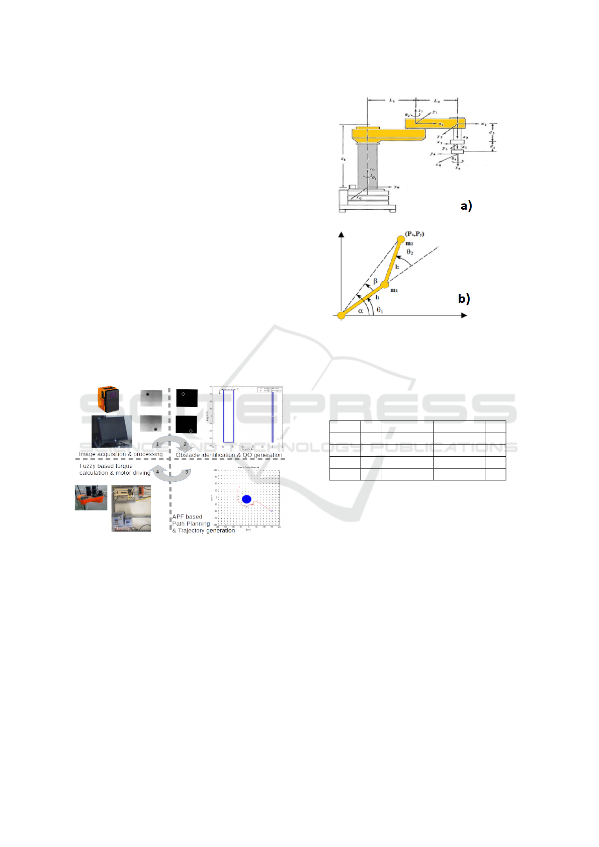
3 THEORETICAL BACKGROUND

3.1 Overall System View

The overall system view is shown in the diagram il-

lustrated in Figure 2. Starting from top-view image

acquisition by a PMD 3D Effector camera from ifm

electronic gmbh

and some digital image processing

techniques in a computer, the obstacle is identiﬁed in

a given scene and represented as circle object. Then,

the region it occupies in cartesian space is mapped to

generate the prohibited conﬁguration space, thus al-

lowing the use of APF to ﬁnd a free-collision path to

the goal point. A smooth trajectory is then calculated

and sent via OPC communication link to the Fuzzy

controller embedded in the PLC for driving the mo-

tors accordingly. This is repeated until goal point is

reached by the manipulator end-effector.

The industrial robot used in this experiment is a

retroﬁtted 4-DOF SCARA, from Toshiba

, whe-

reas the robot playing the role of moving obstacle is

a Zumo Robot from Pololu Robotics and Electronics

. The PLC is a TwidoSuite from Schneider Electric

.

Figure 2: Overall view of the closed-loop system.

3.2 Manipulator Kinematics

In the experiments to be discussed next, only planar

movements were investigated. This was due to lack of

enough driving units for the whole set of 4 joint mo-

tors, what limited the path planning to 2D space only.

However, for completeness, in the following the full-

set of Denavit-Hartenberg (DH) parameters for direct

kinematics, as well as the equations for inverse kine-

matics are reported.

Figure 3 shows the various robot parameters and

frame assignment according to DH convention. As

seen in the illustration, joints 1, 2 and 4 are rotatio-

nal, whereas joint 3 is a prismatic one. Table 1 brings

Figure 3: Illustration of the SCARA manipulator: a) with

assigned references frames; b) in-plane projection of prin-

cipal revolute joints.

the values of the whole set of parameters needed for

deriving kinematic equations.

Table 1: DH parameters of the manipulator.

Axis θ

1 θ

= 0.32 L

= 0.35 0

2 θ

0 L

= 0.30 π

3 0 d

0 0

4 θ

0 0

The adopted convention and the above parameters

allow for obtaining the homogeneous transformation

matrix relating initial and ﬁnal frames as:

T =







0 T

−S

0 T

0 0 −1 T

0 0 0 1







(1)

where : S

= sen(θ

+θ

) , C

= cos(θ

+θ

), T

, T

= l

and T

= d

−d

3.3 SISO Closed-loop Fuzzy Control

Manipulators driven by electric motors usually counts

on reduction gears based transmission system to im-

prove torque and for reducing speed. If on one side

it raises costs, the amount of parts and the rotating

inertia, on the other side it may lead to improved po-

sitioning since the links can undergo displacements of

Can Artiﬁcial Potentials Suit for Collision Avoidance in Factory Floor? - A Case Study of Harmonic Machine-machine Coexistence

549

small magnitude. As discussed in (Spong, 2006), ma-

nipulators having that driving characteristic may be

treated as a SISO system since the gear ratio, β be

among 20 and 100, in such a way that load inertial ef-

fects may be neglected, thus allowing for independent

control (Mittal and Nagrath, 2003). For the manipula-

tor of the present work, whose actuating units are ba-

sed on permanent magnet electric motors with no slip,

an experiment was performed to estimate the gear ra-

tios at the joints, β

and β

. By setting the frequency

inverter to3 Hz, the time required for the joint to com-

plete a 90

rotation was recorded and the number of

revolutions of the motor axis was estimated (see, for

instance, (Fitzgerald et al., 2014)), thus yielding the

ratios presented in Table 2. In the table, the symbol #

stands for “the number of revolutions of”.

Table 2: Data collected from gear ratio estimation.

Joint Time #Motor #Joint β

1 13.35 20.025 0.25 β

= 80.1

2 8.60 12.897 0.25 β

= 51.6

The above calculated gear ratios justify the adop-

tion of joint independent control, and then a SISO

zero-order Takagi-Sugeno Fuzzy controller was de-

signed for each joint (Farooq et al., 2011). The only

reason for adopting this strategy instead of classical

PID or even hybrid PID-Fuzzy is that in our preli-

minary studies, the proposed Fuzzy-TS showed to be

superior in accuracy and repeatability measurements

done according to (ISO, 1998). For what concerns the

controller design itself, most of it relied on theoretical

concepts as well as authors’ experience in manipula-

tor control and agreed with the independent work of

(Nawrocka et al., 2014). As input variables, the joint

position error was calculated from the difference be-

tween desired and measured angular position; it was

limited to the interval [-30;30] in units of internal CLP

memory, what means [-2.63

; 2.63

]. Those values

are in accordance with the positioning-task purpose

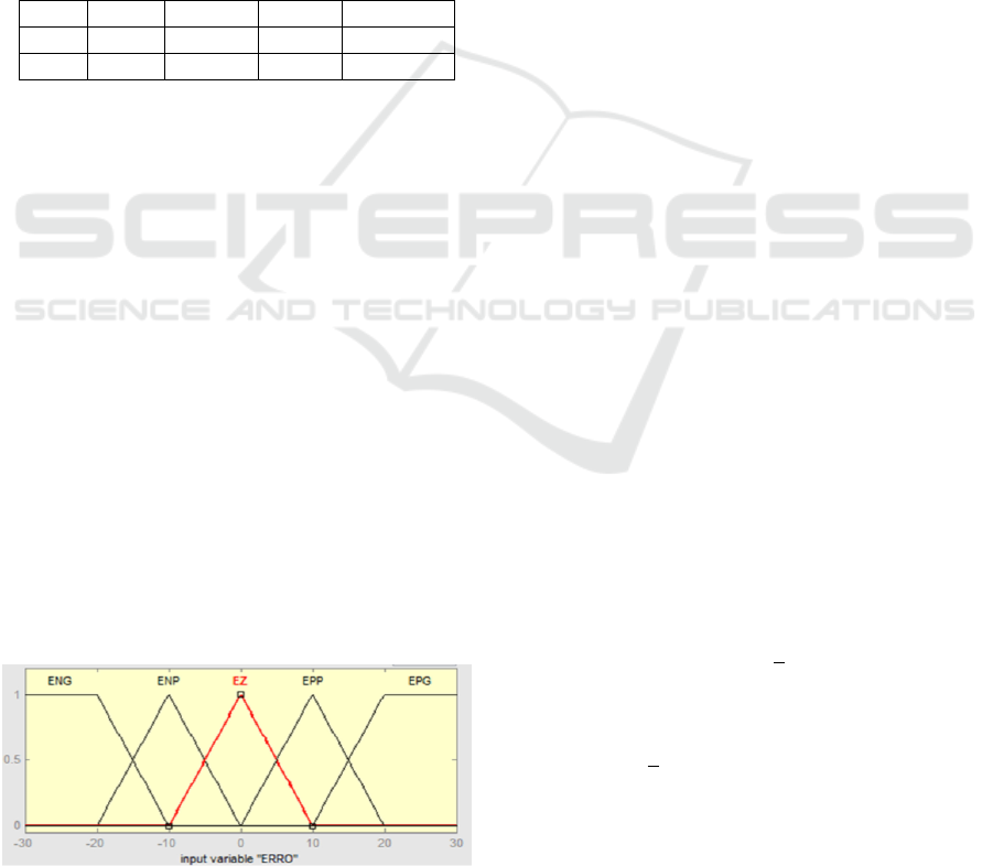
of this experiment. The error fuzzy variable following

the defuzzying step is deﬁned from ﬁve membership

functions, chosen among trapezoidal- and triangular-

like choices as represented in:

Figure 4: Adopted membership functions for input variable

error.

The choice for these simples functions is due to

the limited programming resources in the PLC availa-

ble to host the Fuzzy controller. In addition, the sym-

metry around the origin as well as the 50% overlap

among adjacent functions makes simpler the ladder

enconding of the proposed controller, since the deno-

minators at the defuzzying step get to unity while fa-

vouring the triangle functions to be replaced by linear

parts (Simoes and Shaw, 2007).

Concerning the output variable generated by the

Fuzzy controller, the following constants are deﬁned:

K1=-10, K2=-5, K3=0, K4=5 e K5=10; they respecti-

vely encode the fuzzy variables TNG, TNP, TZ, TPP,

TPG. The interval [-10;10] for the output is associ-

ated to the 0-10V analog range of the PLC output

used to for motor driving, with positive or negative va-

lues yielding clockwise or anticlockwise rotation di-

rection, respectively. The adopted interval also pre-

vents actuator saturation. Finally, ﬁve very simple

fuzzy rules were adopted for the position control task:

If EPG then TNG; If EPP then TNP; If EZ then

TZ; If ENP then TPP; If ENG then TPG;

3.4 Integration of APF to the Control

System

In a few words, artiﬁcial potential ﬁeld method for

free-collision robot motion relies on the existence of

artiﬁcial repulsive potential ﬁelds caused by obsta-

cles, U

rep

(q), and artiﬁcial attractive potential ﬁeld

centered at the target (ﬁnal) position, U

att

(q), guiding

the robot according to the experienced virtual force:

F(q) = −∇U(q), (2)

where

U(q) = U

rep

(q) +U

att

(q). (3)

Usual choices for these potential consider functi-

ons having ﬁrst derivative continuous and smoothly

changing. In the experiments reported here, the at-

tractive potential was built by combining the conical

and parabolic functions (Volpe and Khosla, 1990):

atr

(θ) = dK

k θ − θ

k −

: k θ − θ

k> d,

(4)

atr

(θ) =

k θ − θ

: k θ − θ

k≤ d, (5)

where K

is a constant, θ is the joint position at a

given time instant and θ

is the desired joint position

at the goal point; d deﬁnes the transition limit between

conical and parabolic actions. The parameters are set

= 1 and d = 2cm in the experiments reported here.

ICINCO 2018 - 15th International Conference on Informatics in Control, Automation and Robotics

550

The repulsive potential, in turn, resembles the fol-

lowing ﬂat-sided function:

rep

(θ) =

[

p(θ)

−

]

: p(θ) ≤ p, (6)

rep

(θ) = 0 : p(θ) > p, (7)

in the above equations, K

is a constant, p(θ) re-

presents the minimal distance between the joint posi-

tion , θ, and the whole conﬁguration space of a given

obstacle, QO. At last, p deﬁnes a limit line in conﬁgu-

ration space where the robot can not feel the presence

of that obstacle.The parameters are set K

= 5000 and

p = 2cm in the experiments reported here.

The present implementation of the APF in the pre-

sent work counted on the use of an image sensor for

continuous capture of the scene; this allowed, in turn,

for the calculation of the QO-space in continuous ope-

ration and the generation of free-collision paths. To

calculate the QO-space, an image processing algo-

rithm was developed for detection and localization of

the wheeled robot; robot speed was limited to miti-

gate the effects of the delay between wheeled robot

detection and the manipulator decision on movement

update. Clearly, the events deﬁne the time window

in which the artiﬁcial potential ﬁeld estimates a free-

route.

As it will become clearer in section 3.5, this im-

plementation of APF considered different levels of

description for the manipulator and for the wheeled

robot, namely as a point or an extended body. For

what concerns the manipulator, considering it as a

point has the consequence of applying APF equations

for repulsive ﬁeld between the end-effector only and

the obstacle, whereas when taken as a body, the re-

pulsive potential accounts for the interaction between

the obstacle and many different points throughout the

arm (known as control points).

Things are similar for wheeled robot: when taken

as a point, the repulsive potential is calculated accor-

ding to its distance to the manipulator end-effector (if

this is taken as a point) or to the various control points.

On the other side, if the wheeled robot is regarded as

a body, a line circle centered at its centroid coordina-

tes plays the role of obstacle and, hence, spatial sam-

pling along this line deﬁnes several control points, as

well. This ultimately augments the obstacle space,

since each of the control points now work as a diffe-

rent obstacle.

From this discussion, it should be clear that the

APF computation is highly demanding in the body-

body scenario mentioned latter in this paper.

3.5 Investigated Scenarios

Eight scenarios were designed to study the hypothe-

tical transport experiment reported in this paper. To

compose this set of scenarios two main reasoning li-

nes were followed; one of them regards the geometry,

i.e., the dimensions of both robots, whereas the other

is about the accomplishment of the task itself.

The APF was originally conceived for automatic

motioning in which the mobile robot is generally ta-

ken as a point. Same story for the manipulator; usu-

ally the end-effector is the only portion of the robot

subject to the potential ﬁelds. But what if they are

treated as extended bodies, i.e., their actual dimensi-

ons are not neglected? Roboticists know that the com-

plexity of APF algorithm grows with the deﬁnition of

control point along the manipulator open-chain and

with the number of contact points in the surface of an

obstacle (or, similarly, with the amount of them).

The other issue regards the accomplishment le-

vel of the transport mission: is position uncertainty

acceptable in placing task? Although precision robo-

tics is a very attractive ﬁeld in its own, many industrial

processes do not impose strict constraints for position

or orientation of objects; therefore, reaching a zone

instead of a speciﬁc location may sufﬁce sometimes.

Those arguments were essential to propose the

methodology adopted so far; on one hand, it consists

of describing the robots as a point (P, for short) or as

an extended body (B, for short), thus giving 4 com-

binations for the couple (manipulator robot, wheeled

robot): (P,P); (P,B); (B,P); (B,B). On the other hand,

for what concerns the task itself, two missions were

considered according to the degree of task accom-

plishment: mission-T (target) and mission-Z (zone).

By mission-T it is meant the manipulator task which

requires the object be placed at a speciﬁc point at the

goal, whereas the mission-Z is less restrictive in the

sense that the object may be left in the vicinity of the

goal position (10 cm around the goal was adopted in

the experiments).

3.6 Measuring Task Efﬁciency

To assess the efﬁciency of the manipulator in repe-

atedly doing the hypothetical pick-place task illustra-

ted in Figure 1, the eight scenarios just described were

investigated. On doing that, two measures have been

considered to quantify the efﬁciency of the repetitive

pick-place, which will be described in the following.

3.6.1 Proposed Efﬁciency

In order to quantitatively assess the efﬁciency of the

robotic system in the pick-&-place task, we proposed

Can Artiﬁcial Potentials Suit for Collision Avoidance in Factory Floor? - A Case Study of Harmonic Machine-machine Coexistence

551

a simple equation taking into account the productivity

itself, the variability of time elapsed in each repetition

of the task and the amount of collision events as well.

This function is a ﬁgure-of-merit and works somehow

as an indicator of the inﬂuence of the APF method on

the considered hypothetical process, and that is why

it is named efﬁciency, η. The proposed efﬁciency is

proportional to what we call productivity and inver-

sely proportional to the variance of the elapsed time

and to the number of collisions, according to:

η =

rod

temp

col.

, (8)

where P

rod

is the productivity, which means the

number of times the mission was successfully com-

plete, i.e., the transport from origin to goal did not

suffer any collision, σ

time

is the variance of the time

spent in every repetition of the transport and N

col

the amount of collisions recorded.

3.6.2 Overall Equipment Effectiveness

Although its simplicity, the proposed formula for task

efﬁiciency is not usual in industry. More adequate

is the use of measurements derived from the total

productive maintenance (TPM), originally developed

in Japan for preventing wastes and reducing non-

programmed stops, thus ensuring quality and cost

save in continuous processes. One example is the

Overall Equipment Effectiveness (OEE) (Kennedy,

2017), which is a measure of manufacture systems

for equipment evaluation relying on its performance,

availability and quality. In the following it is dis-

cussed how to interpret the hypothetical pick-&-place

problem in order to measure the robotic system efﬁ-

ciency using this OEE concept.

Availability: its a percentage of the time spent

in effective working condition compared to the total

time available for operation, and is calculated as it fol-

lows:

vail

(%) =

T TD − PP −PNP

T T D − PP

∗ 100, (9)

where TDD is the total time available for opera-

tion, PP is the time reserved for programmed stops

and PNP is the time spent in non-programmed stops.

In the experiments reported in this work, we conside-

red no programmed stops at all; in addition, we asso-

ciate the non-programmed stops to the interruptions

due to collision prevention actions of the manipulator

or to some set-up adjustment. Then, to calculate the

availability, TDD and PNP were both recorded.

Performance: it consists in a relation between

the quantity of parts really produced by the machine

and the expected amount, when considering the cycle

time. In other words, it measures the production rate

of a given equipment, and is calculated as it follows:

er f

(%) =

T EO

∗ 100, (10)

where TEO is the operating effective time and TO

is the operating time. To calculate the performance

in the present work, we considered TO as the time

in which the manipulator was in movement, since the

operation here is regarded as transport rather than fa-

brication itself; the other parameter, TEO, was com-

puted also as a time-in-movement parameter, but pro-

vided exclusion of unsuccessful mission repetitions

(e.g., with collision events).

Quality: it refers to the existence of defective

products ultimately resulting in rejection or rework.

Since in the experiments we have done so far there is

no fabrication at all, we considered the quality, Q

uali

at 100% in equation 11 below.

OEE indicator: it is expressed as the product of

the three metrics just deﬁned according to

OEE(%) = A

vail

∗ P

er f

∗ Q

uali

∗ 100 (11)

3.7 Required Energy Estimation

Also the torque and required energy were estimated in

the various tests performed. A look at the energy con-

sumption is important because it may inﬂuence the

decisions at the factory level. As any problem in en-

gineering, it is pursued a good trend between the be-

neﬁts of new approaches for manufacturing and the

additional costs brought. This could help answering

the following questions: a) can the factory afford the

adoption of an automatic collision avoidance system?

Is the raising of energy costs acceptable? Is the pro-

ductivity increase worth the rise of energy consump-

tion?

In doing this analysis, it has been seen that joint

1 showed superior power demand respect to joint 2.

For this reason, in the tables reporting those quan-

tities, only joint 1 numbers will be presented. Tor-

que and energy calculations followed the approach of

(Fitzgerald et al., 2014) and will be summarized in the

following.

Initially, we take an estimation of the torque at

joint motor 1, T

from:

= 9.55

, (12)

where P

is the nominal power in W coming from

plate speciﬁcations and N

is the rotating speed in

min

-1

. The values for rotating speed were obtained

from the PLC output sent to the frequency inverter

ICINCO 2018 - 15th International Conference on Informatics in Control, Automation and Robotics

552

driver. Since this is a permanent magnet synchrou-

nous motor, it shows no slip and, as such, its rotating

speed can be determined from:

120 f

, (13)

where f is the frequency inverter driver output and

is measured in Hz, whereas P is the number of poles.

Solving equation 12 for the developed power and

using the derivative of angular position at joints as a

measure for the rotating speed, one can use the follo-

wing equation to estimate the power in kW:

9549.2965

, (14)

where T

comes from equation 12 and V

is the

estimation for the joint 1 rotating speed from encon-

ders. The required energy, E, can then be estimated

by integrating the developed power over time, P

E =

∑

i=1

m1i

). (15)

4 RESULTS AND DISCUSSION

For every scenario described in section 3.6, they were

recorded the number of mission repetitions and re-

spective elapsed time, amount of collision events,

number of interruptions due to collision prevention

and the number of accomplished missions (producti-

vity). Those quantities were then used to calculate

the task efﬁciency according to the formulae presen-

ted earlier are reported in Table 3. It is worth menti-

oning that also the time spent during the interruptions

for preventing collisions were recorded.

A look at the table reveals that the scenario (P;B)

led to better productivity and less collisions for both

missions considered. Also interesting to note that no

manipulator stop was observed. The scenario (B;B)

instead led to low productivity, though only one col-

lision event has occurred; interestingly, there were

events of manipulator stops to avoid collision, though

the mission was not accomplished in those rounds.

This may be connected to the artiﬁcial potential ﬁeld

method: since the manipulator is here a extended-

body, the obstacle conﬁguration space gets larger, and

hence the algorithm can not ﬁnd a free-space towards

push the manipulator to end the mission. For what

concerns the efﬁciency of task accomplishment, re-

sults reveal that in the scenarios considering the ma-

nipulator as extended-body the efﬁciency falls; we as-

sociate this to the same lack of free-space just discus-

sed.

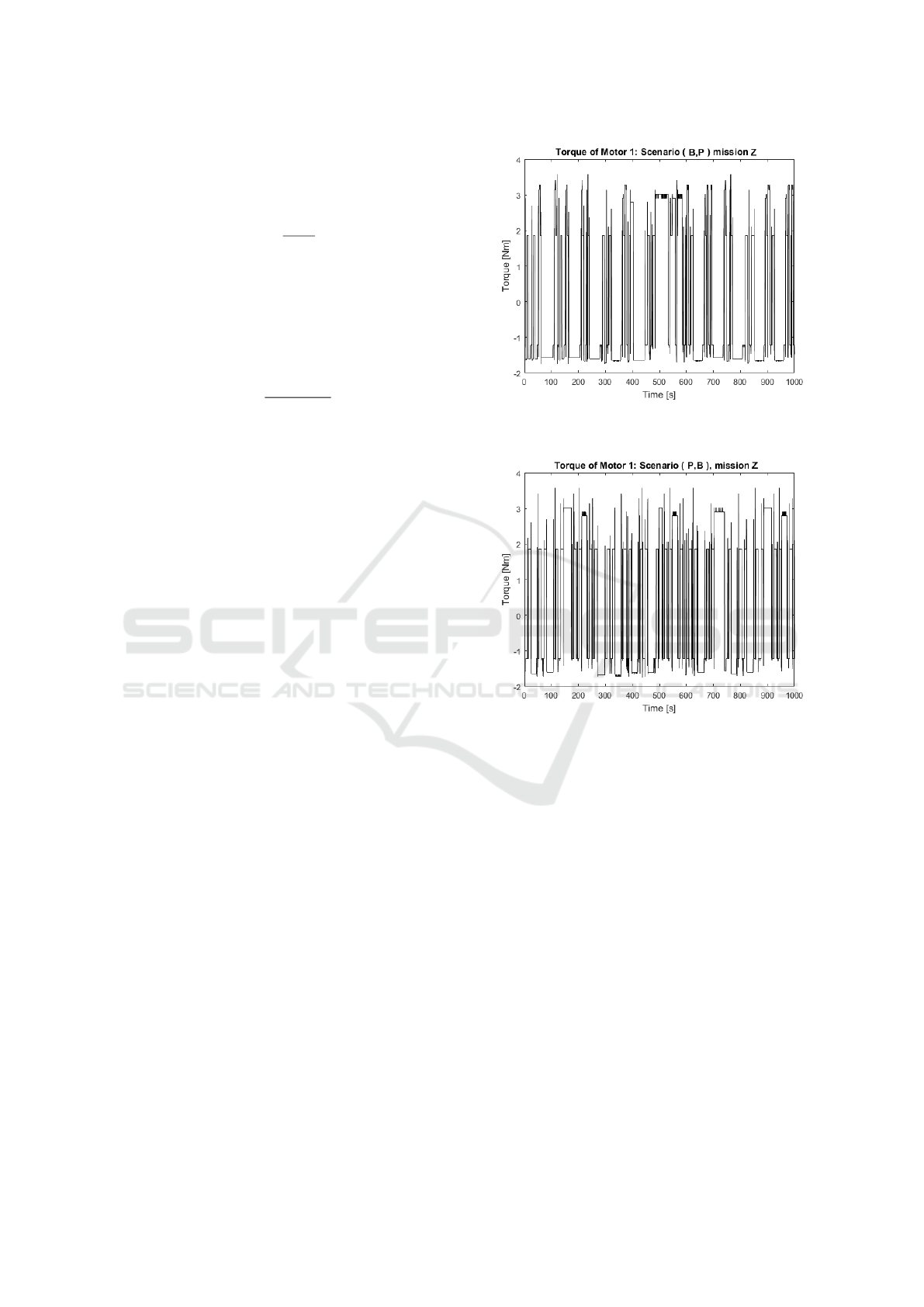
Figure 5: Time-series for motor 1 torque [Nm] in scenario

(B,P), mission-Z.

Figure 6: Time-series for motor 1 torque [Nm] in scenario

(P,B), mission-Z.

In the scenario (P;P) the manipulator is again re-

garded as a point, but, this time, collision events raise.

This is because in this scenario also the obstacle is

considered as a point, what means that the repulsive

ﬁeld pushing the manipulator away is weaken. This

ultimately led to low task efﬁciency.

Using now the OEE indicator as efﬁciency mea-

sure, we could see that results agreed. The scena-

rio (P;B) reached 67.47% and 67.82% for missions-T

and -Z, respectively. We believe the tiny advantage of

mission-Z is because it imposes less constraints to the

artiﬁcial potential ﬁeld method, speeding up the pro-

cess as whole. According to (Kennedy, 2017), those

numbers fall withing the interval [65% - 75%] for the

OEE, making them acceptable, though the universal

recommendations point to 85% as a goal.

Switching the attention to the required energy, re-

sults in the table show more demand in the scenario

(P;B) for both missions. We associate this to the mo-

tor excitation along time, as reported in Figures 5 and

Can Artiﬁcial Potentials Suit for Collision Avoidance in Factory Floor? - A Case Study of Harmonic Machine-machine Coexistence

553

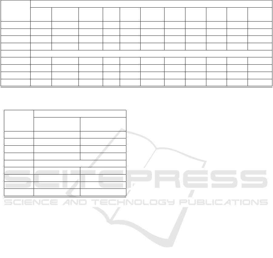
Table 3: Summary of experimental results in the different scenarios evaluated.

Scenario

Mission-T

Trials Time [s] Bumps

rod

Stops η σ

vail

er f

OEE

[%]

Energy

[kW h]

(B,B) 27 182.42 3 20 4 1.333 4.989 59.08 74.92 44.27 0.0041

(B,P) 29 171.04 6 18 5 0.704 4.258 60.00 70.84 42.71 0.0032

(P,B) 36 230.36 5 31 0 8.324 0.744 76.99 87.64 67.47 0.0058

(P,P) 35 198.17 6 29 0 3.491 1.384 42.17 88.37 37.27 0.0042

Scenario Mission-Z

(B,B) 32 207.96 1 27 4 6.921 3.901 40.62 88.95 36.13 0.0037

(B,P) 29 146.70 3 23 3 5.614 1.365 56.62 84.16 47.65 0.0021

(P,B) 35 213.22 3 32 0 12.465 0.855 73.36 92.44 67.82 0.0051

(P,P) 35 210.92 7 28 0 3.303 1.210 73.04 85.07 62.14 0.0040

Table 4: Statistics of the error between desired and real joint

positions.

Scenario

Mission-T

Mean (std dev)

joint 1

Mean (std dev)

joint 2

(B,B) 3.100 (± 1.017) 2.979 (± 0.995)

(B,P) 0.975 (± 1.677) 3.280 (± 1.159)

(P,B) 1.086 (± 1.360) 4.568 (± 1.899)

(P,P) 1.458 (± 0.985) 4.090 (± 2.593)

Scenario Mission-Z

(B,B) 3.177 (± 1.027) 3.503 (± 1.052)

(B,P) 0.692 (± 1.200) 3.009 (± 1.158)

(P,B) 1.167 (± 1.209) 4.037 (± 2.408)

(P,P) 1.592 (± 1.396) 4.382 (± 2.470)

6: more inversion peaks means clearly that the motor

worked harder, thus leading to high productivity. We

can therefore state that higher productivity and bet-

ter efﬁciency led to high energy demand. The authors

found this discussion relevant because it links the path

planning problem, which is a robotic one, to the ma-

chine maintenance issue. Indeed, higher motor exci-

tation implies higher acceleration and breaking levels

during task operations. This analysis should ultima-

tely inﬂuence the choice among the scenarios consi-

dered in the study.

Finally, we have studied the performance of this

hypothetical pick-place system at low level, i.e., at the

level of trajectory-following in conﬁguration and in

cartesian spaces. The goal here is to check how good

was the designed controller in following the path cal-

culated by the trajectory planner. In other words, we

check here the difference (or error) between the desi-

red and measured values of the joint angular position

along time during the robot operation. Table 4 brings

the average error and its standard deviation for every

scenario considered so far.

For better comprehension, we emphasize that er-

ror measures were calculated over time within a gi-

ven mission, and then over different mission repetiti-

ons. In other words, every time the manipulator star-

ted a transport mission from origin to goal position,

the measured and desired joint position were used to

create a time-vector of residuals. Then, average was

calculated from it, and ﬁnally this number was recor-

ded. Successive repetitions of the pick-&-place mis-

sion gave rise to a new error outcome. After several

mission repetitions, the statitics presented in Table 4

were available.

To illustrate the performance of the designed

Fuzzy controller when aided by the path-planner ba-

sed on artiﬁcial potentials, we chose two antagonic

scenarios concerning the productivity tooking care to

consider different missions. In Figures 7 and 8 we

plot, in cartesian space, the desired and real paths at

different moments of the pick-&-place task. The sce-

narios considered in this part of the experiment were

(B;P) mission-Z in Figure 7 as a low-productivity

sample, and (P;B) mission-T in Figure 8 as a high-

productivity sample. Unlike the analysis of producti-

vity, here the scenario (B;P) showed superior perfor-

mance, revealing that high productivity comes at the

expense of innacurate trajectory-following.

5 CONCLUSIONS

In the present work a hypothetical production pro-

cess with non-cooperative machine interaction was

studied. Based on classical approaches, it consis-

ted in providing a SCARA manipulator with the abi-

lity to prevent collisions in a workspace co-shared by

a wheeled robot following random navigation, thus

emulating what could be referred as conﬂicting tasks.

Main goal of the study was to check the conditions for

safe co-existence yet guaranteeing efﬁcient task ac-

complishment. For that end, different scenarios were

considered and different metrics for task efﬁciency

ICINCO 2018 - 15th International Conference on Informatics in Control, Automation and Robotics

554

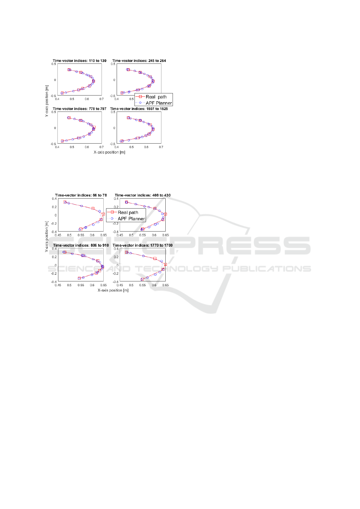
Figure 7: Cartesian space view of free-collision paths in

scenario (B,P) mission-Z, in different repetitions of the

pick-&-place operation. In each plot, blue line refers to the

path generated by the APF planner, and red line refers to the

path really followed by the robot.

Figure 8: Cartesian space view of free-collision paths in

scenario (P,B) mission-T, in different repetitions of the pick-

&-place operation. In each plot, blue line refers to the path

generated by the APF planner, and red line refers to the path

really followed by the robot.

were analyzed. Although this work was not aimed

at providing the scientiﬁc community with a general

procedure for facing the safe co-existence of robots

in industrial environments, we ﬁrmly believe that the

considered case study may result useful for deploy-

ment of such techniques in factory-ﬂoor operations.

Among the various results discussed throughout

the paper, it is worth to highlight that in a path plan-

ning strategy based on artiﬁcial potential ﬁelds, hig-

her task efﬁciency is obtained when the manipula-

tor is described as a point and the obstacle is consi-

dered as extended-body; this favours collision avoi-

dance by keeping robot and obstacle away from each

other while increasing the productivity due to better

workspace usage. A second consequence of this sce-

nario is that the low occurrence of collision events and

non-programmed stops led to less ﬂuctuation in mis-

sion times, thus implying in more productive robot

operation.

According to metrics commonly used in process

and fabrication management, the hypothetical process

emulated in this study reached acceptable levels of

effectiveness, since the estimated OEE amounts to

about 68%. This study could motivate engineers and

practitioners to consider new paradigms about the co-

existence of moving machines in factory ﬂoor.

ACKNOWLEDGEMENTS

Authors thank the Fundac¸

ao N

ucleo de Tecnologia In-

dustrial do Cear

a for administrative facilities.

REFERENCES

Ataka, A., Qi, P., Liu, H., and Althoefer, K. (2016). Real-

time planner for multi-segment continuum manipula-

tor in dynamic environments. 2016 IEEE Internatio-

nal Conference on Robotics and Automation (ICRA),

pages 4080–4085.

Badawy, A. (2014). Manipulator trajectory planning using

artiﬁcial potential ﬁeld. In Engineering and Techno-

logy (ICET), 2014 International Conference on, pages

1–6. IEEE.

Budiyanto, A., Cahyadi, A., Adji, T. B., and Wahyung-

goro, O. (2015). Uav obstacle avoidance using po-

tential ﬁeld under dynamic environment. In Control,

Electronics, Renewable Energy and Communications

(ICCEREC), 2015 International Conference on, pages

187–192. IEEE.

Chatraei, A. and Javidian, H. (2015). Formation control of

mobile robots with obstacle avoidance using fuzzy ar-

tiﬁcial potential ﬁeld. In Electronics, Control, Measu-

rement, Signals and their Application to Mechatronics

(ECMSM), 2015 IEEE International Workshop of, pa-

ges 1–6. IEEE.

Cheng, C., Zhu, D., Sun, B., Chu, Z., Nie, J., and Zhang,

S. (2015). Path planning for autonomous underwater

vehicle based on artiﬁcial potential ﬁeld and velocity

synthesis. In Electrical and Computer Engineering

(CCECE), 2015 IEEE 28th Canadian Conference on,

pages 717–721. IEEE.

Farooq, U., Hasan, K. M., Abbas, G., and Asad, M. U.

(2011). Comparative analysis of zero order sugeno

and mamdani fuzzy logic controllers for obstacle avoi-

dance behavior in mobile robot navigation. In Current

Trends in Information Technology (CTIT), Internati-

onal Conference and Workshop on, pages 113–119.

IEEE.

Fitzgerald, A. E., Kingsley Jr, C., and Umans, S. D. (2014).

Electric Machinery. McGraw-Hill, New York.

Can Artiﬁcial Potentials Suit for Collision Avoidance in Factory Floor? - A Case Study of Harmonic Machine-machine Coexistence

555

Galceran, E., Eustice, R. M., and Olson, E. (2015). Toward

integrated motion planning and control using poten-

tial ﬁelds and torque-based steering actuation for au-

tonomous driving. In 2015 IEEE Intelligent Vehicles

Symposium (IV), pages 304–309. IEEE.

Gayle, R., Sud, A., Lin, M. C., and Manocha, D. (2007).

Reactive deformation roadmaps: motion planning

of multiple robots in dynamic environments. In

Intelligent Robots and Systems, 2007. IROS 2007.

IEEE/RSJ International Conference on, pages 3777–

3783. IEEE.

Guan, W., Weng, Z., and Zhang, J. (2015). Obsta-

cle avoidance path planning for manipulator based

on variable-step artiﬁcial potential method. In The

27th Chinese Control and Decision Conference (2015

CCDC), pages 4325–4329. IEEE.

Habib, M. K. (2014). Handbook of Research on Advance-

ments in Robotics and Mechatronics. IGI Global.

Hargas, Y., Mokrane, A., Hentout, A., Hachour, O., and

Bouzouia, B. (2015). Mobile manipulator path plan-

ning based on artiﬁcial potential ﬁeld: Application on

robuter/ulm. In 2015 4th International Conference on

Electrical Engineering (ICEE), pages 1–6. IEEE.

IFR (2017). Executive summary world robotics 2017 indus-

trial robots: How robots conquer industry worldwide.

Frankfurt. International Federation of Robotics Press.

ISO (1998). Iso9283: Manipulating industrial robots-

performance criteria and related test methods.

Kennedy, R. K. (2017). Understanding, Measuring, and

Improving Overall Equipment Effectiveness: How to

Use OEE to Drive Signiﬁcant Process Improvement.

Productivity Press, New York, 1st edition.

Khatib, O. (1986). Real-time obstacle avoidance for mani-

pulators and mobile robots. The international journal

of robotics research, 5(1):90–98.

Koppula, H. S. and Saxena, A. (2016). Anticipating human

activities using object affordances for reactive robotic

response. IEEE transactions on pattern analysis and

machine intelligence, 38(1):14–29.

Mac, T. T., Copot, C., Hernandez, A., and De Keyser, R.

(2016). Improved potential ﬁeld method for unknown

obstacle avoidance using uav in indoor environment.

In 2016 IEEE 14th International Symposium on Ap-

plied Machine Intelligence and Informatics (SAMI),

pages 345–350. IEEE.

Mittal, R. and Nagrath, I. (2003). Robotics and control. Tata

McGraw-Hill.

Moellmann, A. H., Albuquerque, A. S., Contador, J. L.,

and Marins, F. A. S. (2006). Aplicac¸

ao da teoria das

restric¸

oes e do indicador de eﬁci

encia global do equi-

pamento para melhoria de produtividade em uma linha

de fabricac¸

ao. Revista gest

ao industrial, 2(1).

Mora, M. C. and Tornero, J. (2008). Path planning and

trajectory generation using multi-rate predictive arti-

ﬁcial potential ﬁelds. In Intelligent Robots and Sy-

stems, 2008 IEEE/RSJ International Conference on,

pages 2990–2995. IEEE.

Nawrocka, A., Nawrocki, M., and Kot, A. (2014). Fuzzy lo-

gic controller for rehabilitation robot manipulator. In

Control Conference (ICCC), 2014 15th International

Carpathian, pages 379–382. IEEE.

Pinto, L., Davidson, J., and Gupta, A. (2016). Supervision

via competition: Robot adversaries for learning tasks.

arXiv preprint arXiv:1610.01685.

Simoes, M. G. and Shaw, I. S. (2007). Controle e Modela-

gem Fuzzy. Edgard Blucher, Sao Paulo, 2nd edition.

Spong, M. W. (2006). Robot modeling and control, vo-

lume 3. Wiley New York.

Volpe, R. and Khosla, P. (1990). Manipulator control with

superquadric artiﬁcial potential functions: Theory and

experiments. IEEE Transactions on Systems, Man,

and Cybernetics, 20(6):1423–1436.

Wang, X., Jin, Y., and Ding, Z. (2015). A path planning

algorithm of raster maps based on artiﬁcial potential

ﬁeld. In Chinese Automation Congress (CAC), 2015,

pages 627–632. IEEE.

Yu, K., Ohnishi, K., Kawana, H., and Usuda, S. (2015a).

Modulated potential ﬁeld using 5 dof implant assist

robot for position and angle adjustment. In Industrial

Electronics Society, IECON 2015-41st Annual Confe-

rence of the IEEE, pages 002166–002171. IEEE.

Yu, K., Uozumi, S., Ohnishi, K., Usuda, S., Kawana, H.,

and Nakagawa, T. (2015b). Stereo vision based ro-

bot navigation system using modulated potential ﬁeld

for implant surgery. In Industrial Technology (ICIT),

2015 IEEE International Conference on, pages 493–

498. IEEE.

ICINCO 2018 - 15th International Conference on Informatics in Control, Automation and Robotics

556