
OSPF Algebraic Formal Modelling using ACP
A Formal Description on OSPF Routing Protocol
Pedro Juan Roig
1,2
, Salvador Alcaraz
1
, Katja Gilly
1
and Carlos Juiz
2
1
Department of Physics and Computer Architecture, Miguel Hernández University, 03202 Elche (Alicante), Spain
2
Department of Computer Science, University of the Balearic Islands, 07122 Palma de Mallorca, Spain
Keywords: ACP, Formal Protocol Specification, Networking, OSPF.
Abstract: OSPF may well be the most popular routing protocol within Autonomous Systems, being used in all kind of
networks around the world. In this paper, we first design a basic model by focusing on the main tasks of a
router running OSPF, hence being neighbour discovery and a simplified route management, by means of
algebraic derivations using Algebra of Communicating Processes (ACP). Taking this model as a base case
scenario, we extend it by adding up some timing behaviour present in real OSPF implementations and by
detailing the packet exchanges involved in route management.
1 INTRODUCTION
We are living in an ever increasingly networked
world and routing protocols are key players in
supporting network communications. Focusing on
the OSI model (X200, 1994), communication among
network devices are mainly performed at layer 3,
namely, network layer.
As far as network communication is concerned,
layer 3 protocols are run in all interconnection
devices that belong to any network, providing an end
to end communication. Network communication
tasks are usually performed by routers, although it
might also be done by any layer 3 device with the
proper software package, such as switches, firewalls
or devices with multiple network adapters.
Those layer 3 devices communicate with each
other through routing protocols in order to exchange
their routing updates and build up and maintain their
own routing tables, which contain the best routes to
any attainable network according to common
criteria.
Routing protocols may be classified as Interior
Gateway Protocols (IGP) and Exterior Gateway
Protocols (EGP). A protocol belonging to the former
is implemented within an Autonomous System (AS),
thus among devices being managed by a common
administration, whereas the latter is reserved for
routing among different AS, like BGP.
Within IGP, protocols may be distinguished
between Distance Vector and Link State, the former
ones being like a route post, hence dealing with the
cost to get to a destination and pointing to the next
hop in the way there and the latter ones being like a
route map, thus having the aforesaid features and
also a topology map.
Among Link State protocols, there are two
protocols involved, being Intermediate System to
Intermediate System (IS-IS) and Open Shortest Path
First (OSPF), both standardized by IETF. The
former is mainly used in ISP environments and the
latter is the most widespreadly used, both in IPv4
(RFC 2328, 1998) and in IPv6 (RFC 5340, 2008)
domains. The aim of this paper is to get a realistic
approach model to OSPF behaviour.
The organization of this paper will be as follows:
first, Section 2 introduces formal description
techniques, then, Section 3 shows an OSPF informal
specification, next, Section 4 presents some Algebra
of Communicating Processes (ACP) fundamentals,
after that, Section 5 will get a basic router modelling
in an OSPF environment, afterwards, Section 6 will
render some examples of the basic modelling, later,
Section 7 will perform a detailed router modelling in
an OSPF environment, right after that, Section 8 will
perform a model verification and finally, Section 9
will draw the final conclusions.
2 FORMAL DESCRIPTION
TECHNIQUES
The use of Formal Description Techniques (FDT) in
Roig, P., Alcaraz, S., Gilly, K. and Juiz, C.
OSPF Algebraic Formal Modelling using ACP - A Formal Description on OSPF Routing Protocol.
DOI: 10.5220/0006838700550066
In Proceedings of the 15th International Joint Conference on e-Business and Telecommunications (ICETE 2018) - Volume 1: DCNET, ICE-B, OPTICS, SIGMAP and WINSYS, pages 55-66
ISBN: 978-989-758-319-3
Copyright © 2018 by SCITEPRESS – Science and Technology Publications, Lda. All rights reserved
55

order to study the ever growing complexity of
concurrent communication protocols is increasing as
it provides unambiguous descriptions in a more
precise way than any description made in natural
languages.
Because of that degree of complexity, there is
not a universal FDT to be employed in all cases but
it is necessary to deal with some of them, such that
one might better fit in some case scenario whereas
another one might do it in another situation.
Among all FDT, some of the tools most
commonly used tools are ESTELLE, LOTOS and
SDL (Turner, 1993). Otherwise, Petri Nets (Petri,
1966) are also widely used, as well as FSM and
Promela.
Eventually, Process Algebras may also be used
for that purpose, and among them, ACP (Bergstra
and Klop, 1985) might be one of the best suited for
dealing with distributed and concurrent systems, as
it abstracts away from the real nature of a system,
thus presenting it as a set of equations according to
its behaviour. The aforesaid equations are related to
the ACP axioms and processes are the solutions of
such systems of equations (Padua, 2011).
All Process Algebras share the concept of
Labelled Transition Systems (LTS) in order to
specify behaviour equivalence. Such systems are
formed by states whose transitions among them are
labelled with the proper associated actions. This
makes possible to model concepts regarding
distributed processing systems, such as OSI services
and protocols.
ACP is going to be used in order to get a formal
specification of OSPF, but before proceeding with it,
an OSPF informal specification will be presented so
as to later model those relevant features using ACP.
This work is going to extend a previous study on
formal description of OSPF by means of ACP (Roig
et al., 2018).
3 OSPF INFORMAL
SPECIFICATION
All routing protocols perform three basic functions,
such as identifying their neighbours on the network,
managing the route paths to all possible destinations
and making dynamic decisions as to where to
forward user traffic coming in. Those three actions
are necessary to build up and maintain the routing
table, thus forming control plane operations. Once
the routing table is completed, data plane will take
advantage of it in order to forward user traffic.
The first function may be known as neighbour
discovery and all OSPF routers exchange hello
messages through all their OSPF interfaces in order
to identify all their OSPF neighbours. All devices
within the same OSPF area must have the same hello
and dead timers, the same type of authentication, if
any, and the logical addressing of each interface
must be coherent with that of their link neighbours.
If this is the case, an OSPF neighbour relationship
will be established.
The second function may be known as route
management and all OSPF routers exchange routing
update messages in order to keep track of all
possible destinations available within the OSPF
environment.
In order to implement both functions, OSPF does
not use any transport protocol, such as TCP or UDP,
but it carries the data directly through an IP packet,
using protocol number 89 as the IP protocol field in
the IP header.
OSPF has five different types of packets, carried
inside an IP packet, whose functions are described in
Table 1.
Table 1: OSPF packet types.
Type Packet name Function
1 Hello
Discovering and maintaining
neighbors
2
Database
Description
Exchanging Data Base route
headers
3
Link State
Reques
t
Requesting Data Base route
updates
4 Link State Update
Sending Data Base route
updates
5 Link State ACK
Sending Acknowledgments to
route updates
Therefore, each local router running OSPF
implements the neighbour discovery function by
exchanging OSPF type 1 packets with all its OSPF
neighbouring routers, whereas the route
management function is performed by exchanging
the rest of OSPF packets types in the proper way.
As OSPF is a link state routing protocol, it holds
a Link State Data Base (LSDB) containing all routes
to all networks within the OSPF domain.
Furthermore, it implies all routers must have their
LSDB synchronised, meaning that all of them must
share the same information about the network
topology after the necessary route exchange, before
achieving the state of convergence. OSPF is a fast-
converging routing protocol, such as a network
composed by a few routers may converge just in a
few seconds.
Regarding router management, when a local
router has knowledge of any new route or a route
update, it sends an OSPF type 2 packet to its proper
DCNET 2018 - International Conference on Data Communication Networking
56
OSPF neighbouring routers. Those packets are also
known as Data Base Description (DBD) and they
contain a set of the route headers regarding those
routes. Upon receipt of a DBD, those OSPF
neighbouring routers check whether each route
header present within a DBD is also present within
their LSDB.
LSDB keeps not only the route headers but full
data about routes, allowing the buildup of a network
topology. Each LSDB entry belongs to a single route
and it is called Link State Advertisement (LSA).
Therefore, DBD packets contain summaries of the
LSA. Actually, the sending and receiving DBD is
called DataBase Exchange Process, where each LSA
has a sequence number and is acknowledged by
echoing it.
Each LSA header present in a DBD contains
some fields to identify in a unique way an LSA, such
as LS ID, LS type and Advertising Router, but in
order to determine which instance is more recent,
this is, the one inside the incoming DBD or the one
already stored within the LSDB, the fields to be
examined are LS Sequence Number, LS Age and LS
Checksum.
When a local router detects an LSA more recent
than its own database copy, then it sends an OSPF
type 3 packet to the OSPF neighbouring router
which sent that particular OSPF type 2 packet, so as
to request an update and in turn an OSPF type 4
packet will be deliver from that neighbour.
Eventually, each OSPF type 4 packet will be
acknowledged by an OSPF type 5 packet.
In addition to it, OSPF type 4 packets will be
sent from every local router to all of its proper OSPF
neighbours every 30 minutes by default, this is 1800
seconds, in order for them to refresh their LSA,
although some manufacturers might set different
values varying from 5 to 59 minutes. If such a
refreshment is not produced, the LSA will be flushed
from LSDB if its timer reaches its maximum aging
time, which is 1 hour, this is, 3600 seconds.
Special attention must be paid to OSPF type 4
packets, as those packets implement the flooding of
LSA, containing information about routing, metric
and topology regarding a particular section of the
OSPF network, thus being the relevant stuff about
routing updates. One particular OSPF type 4 packet
may contain a single LSA or multiple LSA.
LSA are used to fill and update LSDB, although
there is not only one sort of LSA but a few of them,
each one being employed for advertising different
OSPF networks. The mostly used LSA types are 1 to
5, although there are defined up to eleven types.
It must be taken into consideration that OSPF is
a highly scalable routing protocol because of the
concept of area, which permits the division of the
whole OSPF domain in different areas, hence routers
belonging to one particular area must have their
LSDB synchronised.
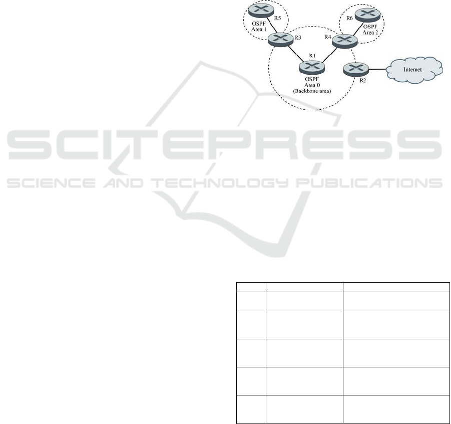
The connection among two or more areas is
performed by an Area Border Router (ABR) which
is a router that has interfaces in more than one area,
thus being able to propagate routes through all of
them. In addition to it, an Autonomous System
Boundary Router (ASBR) is a router being the edge
router with another routing domain, which also
might propagate some external routes inside. Those
OSPF multiarea concepts are depicted in Figure 1.
Figure 1: Multiarea OSPF routing domain.
Regarding LSA types, there are LSA types 1 and
2 that carry routes within the same OSPF area, thus
they are referred to as intra-area LSA. There are also
LSA types 3 and 4 that carry routes from one area to
another one, thus they are known as inter-area LSA.
Finally, there are LSA type 5 that carries external
routes redistributed into OSPF domain.
The mostly used LSA types are described in
Table 2, where the acronym DR will be described in
due course.
Table 2: OSPF LSA main types.
Type LSA name Function
1 Router LSA
Each router advertises all its
directly connected links
2 Network LSA
Each DR in a multi-access
network advertises all the
routers connected
3 Summary LSA
Each ABR advertises routes
from one area into other
connected areas
4 Summary ASBR LSA
Each ABR advertises routes
coming from an ASBR to show
where it is
5 AS external LSA
Each ABR advertises external
routes being redistributed into
OSPF domain
Apart from that, it is important that all
neighbours within a particular network segment
OSPF Algebraic Formal Modelling using ACP - A Formal Description on OSPF Routing Protocol
57
share the same OSPF network type. There are four
main types according to the standards, each of them
having particular characteristics. This fact makes
each of those network types a different case
scenario, as they might be exhibited in the following
points:
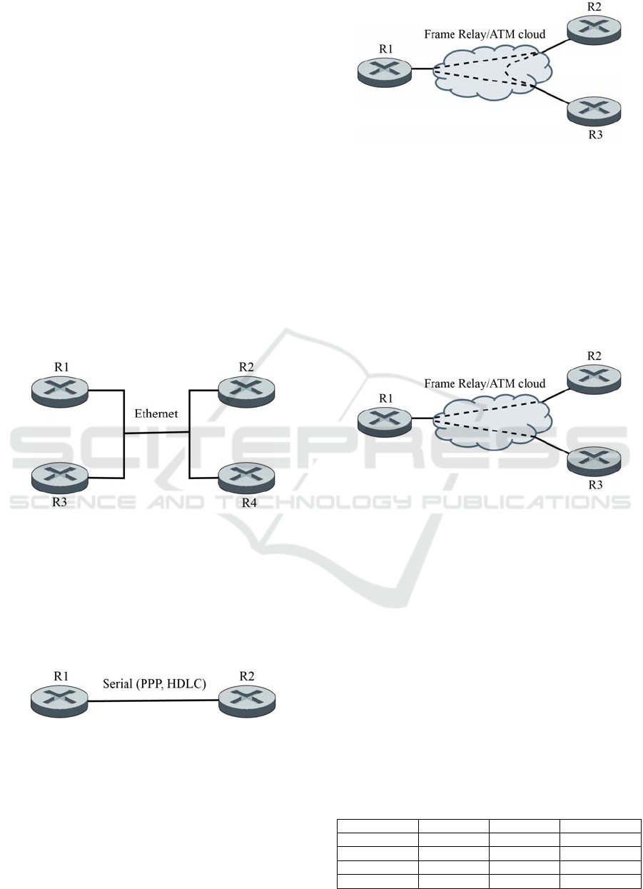
A. Broadcast (BRC)
There might be more than two neighbours within a
single network segment and then a Designated
Router (DR) and a Backup Designated Router
(BDR) must be assigned. The first one will be in
charge of receiving an LSA containing the routing
updates from a given neighbour and sending it back
to the rest of the neighbours, whereas the second one
will keep track of all receiving LSA but will not be
sending anything. With respect of the rest of
neighbours, they will be considered DROthers and
will not share LSA directly with any other
neighbour. The typical example of this network type
is an Ethernet environment, like in Figure 2.
Figure 2: OSPF Broadcast network.
B. Point to Point (P2P)
There are just two neighbours, so there is no need to
appoint a DR or a BDR as they both will be
exchanging LSA. A typical example of this network
type is a Serial link between two pairs, working with
layer two protocols PPP or HDLC, as in Figure 3.
Figure 3: OSPF Point to Point network.
A. Non Broadcast MultiAccess (NBMA)
It is found on non broadcast environments, such as
Frame Relay or ATM, and a multi-access topology
is needed, such as Full Mesh or Partial Mesh. There
might be present more than two neighbours,
therefore a DR and a BDR must be appointed, such
as in Figure 4.
Figure 4: OSPF Non Broadcast MultiAccess network.
B. Point to MultiPoint (P2MP)
It is present on non broadcast environments, such as
Frame Relay or ATM, and a Hub-and-Spoke
topology is implemented. In such a case, that
topology might be considered as a string of point to
point links, as all spokes routers must first
communicate with the hub in order to do it with
another spoke router, so there is pointless to assign a
DR and a BDR, as shown in Figure 5.
Figure 5: OSPF Point to MultiPoint network.
As stated before, neighbour discovery function
implies that all link neighbours share the same
values of hello timers and dead timers. There is a
timer set for each interface. The hello interval is
used to maintain neighbour relationships, thus being
reset upon each sending, whereas the dead interval is
used to delete such neighbour relationship after 4
silent hello intervals and it is reset upon receiving a
hello packet from a neighbour.
The hello interval defines how often a hello
packet is sent over whereas the dead interval sets the
waiting time for a hello packet before the neighbour
is declared dead. The default values of both timers
depend on the network type and they are described
in Table 3.
Table 3: Hello and Dead Timers –vs– Timer Types (TT).
Network Type Hello Time
r
Dead Time
r
Value
BRC 10 sec. 40 sec. TT = 0
P2P 10 sec. 40 sec. TT = 0
NBMA 30 sec. 120 sec. TT = 1
P2MP 30 sec. 120 sec. TT = 1
DCNET 2018 - International Conference on Data Communication Networking
58

In case any two neighbours are exchanging LSA,
an OSPF adjacency relationship will be established.
At that point they will start exchanging a full copy
of their LSDB and in turn they will be sending each
other any given routing update in order to keep their
LSDB synchronised.
Once LSDB belonging to all routers within a
given area are in synchronisation, then the Shortest
Path First (SPF) algorithm, also known as Dijkstra
algorithm (Dijkstra, 1959), will be run in each
router, taking itself as the root of the tree, in order to
get the shortest path tree from each router to all
networks present in the OSPF domain.
The SPF algorithm takes interface bandwidth in
order to calculate its cost, also known as metric. It
must be taken into account that the standard OSPF
v1 was released in the early 90s, so by that time a
FastEthernet link was the fastest and the original
expression to calculate it was the integer part of a
fraction where the numerator was 10
8
and the
denominator was the link bandwidth in bps, being 1
the least possible cost.
Therefore, a FastEthernet 100 Mbps link would
have an OSPF cost of 1 and also any faster link,
whereas a Serial 1.544 Mbps T1 link will have 64.
Later on, that formula was adjusted accordingly but
nowadays it is still considered as the default
implementation for backward compatibility
purposes.
On completion of the Dijkstra algorithm in each
router, the routes with the least cost from a particular
router to all those OSPF domain networks will be
selected and in turn they will be written into the
routing table.
At that stage, the third function exposed above
for any routing protocol will be fulfilled. Therefore,
the routing table will be built up, meaning that the
router will be ready to forward data packets to any
destination within the OSPF domain.
This is an OSPF informal specification, but we
are looking forward to achieving an OSPF formal
specification that captures the protocol behaviour.
4 ACP FUNDAMENTALS
The FDT chosen to model OSPF is going to be ACP,
which is a kind of process algebra that allows to
describe concurrent communication processes in an
abstract way, in a similar fashion as abstract algebras
do.
This is done by getting some ACP process terms
being behaviourally equivalent as the process to be
modelled, hence being OSPF, without caring about
other implementation details of that process being
described.
In order to achieve this, the concept of
bisimulation equivalence is used, also known as
bisimilarity, meaning that two processes may
execute the same string of actions and also have the
same branching structure (Fokkink, 2007).
Therefore, two bisimilar processes are considered to
behave in an equivalent manner.
ACP has its own set of axioms so as to prove that
two process terms have an equivalent behaviour.
Those axioms make use of the syntax and semantics
of ACP operators (Lockefeer et al., 2016).
The basic signature of a framework for ACP
consists of atomic actions, such as sending and
receiving data, which represent actions whose
behaviour may not be further divided, as well as
alternative operators, defined as sums, and
sequential operators, defined as products.
That may be extended with the use of concurrent
operators (||), whose behaviour may be described by
the left merge operator (||_) and the communication
merge operator (|) by means of the Expansion
Theorem, presented by Bergstra and Klop (Bergstra
and Klopp, 1984), where
}{}..{
1 in
i
XXXX
and
},{}..{
1
,
jin
ji
XXXXX
:
ji
ji
i
in
XXXXXXX
,
1
_||)|(_||)||...||(
(1)
Therefore, depending on the number of concurrent
processes, the expression goes this way:
21122121
|_||_||)||(2 XXXXXXXXn
132
231321
213312
321321
_||)|(
_||)|(_||)|(
)||_(||)||_(||
)||_(||)||||(3
XXX
XXXXXX
XXXXXX
XXXXXXn
)||_(||)|()||_(||)|(
)||_(||)|()||_(||)|(
)||_(||)|()||_(||)|(
)||||_(||)||||_(||
)||||_(||)||||_(||
||||||4
21433142
41323241
42314321
32144213
43124321
4321
XXXXXXXX
XXXXXXXX
XXXXXXXX
XXXXXXXX
XXXXXXXX
XXXXn
The behaviour of the left merge and the
communication merge operators is the following:
)||(_||)( yxvyxv
(2)
zyzxzyx _||_||_||)(
(3)
OSPF Algebraic Formal Modelling using ACP - A Formal Description on OSPF Routing Protocol
59

)||()|()(|)( yxwvywxv
(4)
zyzxzyx |||)(
(5)
In addition to it, the encapsulation operator
)(
iH
X
forces internal actions into communication. Joining
it with the concurrent operator shown above, the
outcome will only depend on whether the first factor
of each term belongs to set
H
or otherwise, where
constant
represents a deadlock and the set
H
represents all internal actions related to sending and
receiving messages.
Hvvv
H
,)(
(6)
Hvv
H
,)(
(7)
)(
H
(8)
)()()( yxyx
HHH
(9)
)()()( yxyx
HHH
(10)
For a communication to take place in a channel, a
sending action is needed at one end whereas a
receiving action is needed at the other one, otherwise
deadlock
)(
will happen.
Therefore, communication is going to be
considered herein as unidirectional, hence, regarding
the channel where its sending point is
i
and its
receiving point is
j
:
jijiji
crs
,,,
|
(11)
ijji
rs
,,
|
(12)
lkji
rs
,,
|
(13)
In summary, when applying the encapsulation
operator to the Expansion Theorem in order to
derive concurrent processes, only terms starting with
a communication merge operator having both the
same initial end and the same final end will prevail,
whereas all of the other terms will be discarded.
Furthermore, a conditional operation is declared
in order to distinguish whether a condition has been
accomplished or otherwise. This way, data can
influence process behaviour. As per its syntax, the
condition offers a Boolean data type and goes in the
middle of the expression, surrounded by two
triangles pointing outwards, whereas the True
condition goes ahead and the False condition goes
behind.
FalseConditionTrue ||
(14)
Those are the necessary ACP operators in order
to undertake the modelling of OSPF through
algebraic derivations. According to that, two
different models are presented:
a basic model, making some assumptions over
the OSPF packet exchange in order to keep it as
simple as possible
a detailed model, following the actual OSPF packet
exchange in order to make it as close to real as
possible
5 BASIC ROUTER MODELLING
IN OSPF
The aim of this basic model is to get the big picture
of OSPF dynamics and a couple of assumptions are
to be made for that purpose.
The first one is to take the LSA exchange
process as a whole, thus considering the exchange of
OSPF packet types 2, 3, 4 and 5, as a single process
so as to keep things simple.
It is worth noting that the LSA exchange process
gets the synchronisation of LSDB belonging to all
OSPF routers within the same area so as to
eventually have the same contents within their
respective LSDB. That is why OSPF is considered a
link state routing protocol. At that point, the OSPF
routers are fully adjacent, thus making LSDB
synchronisation process possible in a predictable
time interval.
The second one is to ignore all the timers
involved in OSPF, namely, on one hand, hello timer
and dead timer in order to keep the neighbour
relationships and, on the other hand, the LSA refresh
timer and the max age LSA timer in order to keep
the each LSA entry in LSDB updated.
Keeping those assumptions in mind, a basic
OSPF model will be built up and for that purpose,
we have to deal with the three basic functions
describe in Section 3.
The first function was Neighbour Discovery,
where messages flow in all directions from all OSPF
routers looking for their OSPF neighbouring routers.
Using ACP syntax and semantics, it may be said
that a local OSPF router
i
exchanges hello
messages
)(h
through all its OSPF interfaces,
facing its
j
neighbouring OSPF routers, regardless
of the network type or which area they are located
in.
Therefore, Neighbour Discovery is modelled by
the following expression:
DCNET 2018 - International Conference on Data Communication Networking
60

))()((
,,1_
hrhsR
ij
ij
jii
(15)
When the sending and receiving actions from
neighbouring routers flow through the same channel
in the same direction (the same routers
i
and
j
, in
the same order), hello communication will occur,
therefore:
)()(|)(
,,,
hchrhs
jijiji
(16)
On the contrary, if both actions do not meet the
aforesaid requirements, it will yield deadlock (
).
This will get the expected result, such as
communication will take place between any router
and any of its neighbours, always in a unidirectional
fashion, hence all OSPF neighbours will be engaged
in a neighbour relationship.
The second function was Route Management and
the main difference with the previous one is that
network type is crucial, as LSA will be exchanged
by the routers having an adjacency relationship. It
must be taking into consideration that this basic
model assumes that the aforesaid function is
modelled as a single process.
According to the behaviour of DR and BDR
routers exposed above, the following table shows
whether LSA communication will take place
between a sender and a receiver. The role of each
sender will be shown as rows whereas the role of
each receiver will be seen as columns.
If a cell being the crossing point between a row
represented by a sender and a column represented by
a receiver shows 1, then LSA communication will be
held and LSA will be exchanged. Otherwise, if a cell
shows 0, then LSA communication will not be
produced between that sender and that receiver.
Needless to say that communication between a
single router being both sender and receiver is not
allowed. It all may be appreciated in Table 4.
Table 4: Valid Communication Channels.
r
DR
r
BDR
r
DRO1
r
DRO2
r
DRO3
r
DRO4
s
DR
- 1 1 1 1 1
s
BDR
1 - 0 0 0 0
s
DRO1
1 1 - 0 0 0
s
DRO2
1 1 0 - 0 0
s
DRO3
1 1 0 0 - 0
s
DRO4
1 1 0 0 0 -
In addition to it, it is also necessary to assign
different values to the four different network types
previously defined, depending whether DR and BDR
are appointed or otherwise, as seen in Table 5.
Table 5: Values assigned to network types (NT).
Network Type Nomenclature Value
Broadcas
t
BRC NT = 0
Point to Poin
t
P2P NT = 1
Non Broadcast
MultiAccess
NMBA NT = 0
Point to MultiPoin
t
P2MP NT = 0
In order to implement Table 4 in an equation, it
is first necessary to assign different values to the
different router roles and also keeping in mind the
values given by Table 5. This is shown in Table 6.
Table 6: Values assigned to router roles.
Network
Type
Router
Role
Naming Value
NT = 0 Designated Route
r
DR 3
NT = 0
Backup Designated
Route
r
BDR 2
NT = 0 DR Othe
r
DRO 1
NT = 1 Point to Point Routers - 0
Putting it all together, coefficients
ji
k
,
will be
implemented in order to capture the behavior
exhibited in the previous tables. Those coefficients
have binary values, thus 1 or 0, depending on
whether communication exists in the channel
starting in a router
i
and ending in a router
j
.
Therefore, the coefficients will permit
communication between peers in a unidirectional
way or otherwise.
The role corresponding to the local router
i
will
be carried by variable
x
whereas the role
corresponding to its neighbouring router
j
will be
carried by variable
y
.
Those coefficients take their values from the next
equation, taking the integer part of a fraction
containing the role of both ends of the channel and
the network type:
NT
yx
k
ji
5
2
int
,
(17)
In order to get the roles for each router within each
network type, which will provide
x
and
y
values,
it is necessary to implement an algorithm having all
of the routers within a network segment
)(n
and its
network type
)(NT
as arguments, such as
Algorithm 1.
OSPF Algebraic Formal Modelling using ACP - A Formal Description on OSPF Routing Protocol
61

RouterRole(n,NT){
If (NT == 1)
Then
For (z = 0; z < count(n); z++)
Do
z.Role = 0;
Done
Else
If (NT == 0)
Then
DR.priority = 0;
DR.router-id = 0;
BDR.priority = 0;
BDR.router-id = 0;
Flag = 0;
For (z = 0; z < count(n); z++)
Do
If (z.priority > DR.priority)
Then
DR.priority = z.priority;
DR.router-id = z.router-id;
Flag = 1;
z.Role = 3;
Else
If (z.priority == DR.priority)
Then
If (z.router-id > DR.router-id)
Then
DR.router-id = z.router-id;
Flag = 1;
z.Role = 3;
EndIf
EndIf
EndIf
If (Flag == 0)
Then
If (z.priority > BDR.priority)
Then
BDR.priority = z.priority;
BDR.router-id = z.router-id;
Flag = 1;
z.Role = 2;
Else
If (z.priority == BDR.priority)
Then
If (z.router-id > BDR.router-id)
Then
BDR.router-id = z.router-id;
Flag = 1;
z.Role 2;
EndIf
EndIf
EndIf
If (Flag == 0)
Then
z.Role = 1;
EndIf
Done
EndIf
EndIf
}
Algorithm 1: RouterRole(n,NT).
Using ACP syntax and semantics, it may be said
that a router
i
exchanges LSA messages
)(d
through its proper OSPF interfaces, this is, facing its
j
neighbours where the coefficients given by (17)
are 1 no matter the network type.
Therefore, Route Management is modelled by
the following expression:
))()((
,,,,2_
drkdskR
ijij
ij
jijii
(18)
Analogously as the previous function,
communication will only take place in a
unidirectional fashion between a given sender and a
particular receiver, yielding deadlock (
) in the rest
of the cases.
)()(|)(
,,,
dcdrds
jijiji
(19)
The third function was Path Determination and
consists in making decisions about where to forward
each network message coming in, in other words,
filling up the routing table according to the Shortest
Path First (SPF) algorithm, also known as Dijkstra
algorithm.
Two actions need to be performed in order to
achieve that. The first action is running the Dijkstra
algorithm, considering the OSPF metric as the cost
to be minimised. It solves the problem of finding the
shortest paths from a source node to the rest of the
nodes within a network, providing all edges do have
non-negative weights.
Algorithm 2: Dijkstra(i,G).
A pseudocode algorithm implementing this
action, starting with router
i
as the root of the
shortest path tree for the weighted graph
),( VEG
representing the OSPF domain,
composed by all vertices
Vv
with edges acting
as the weight function
REw :
among those
Dijkstra(i,G){
dist[i] ← 0
for all v ∈ V–{i}
do dist[v] ← ∞
done
S ← ∅
Q ← V
while Q ≠ ∅
do
u ← mindistance(Q,dist)
S ← S ∪ {u}
for all v ∈ neighbors[u]
do
if dist[v] > dist[u] + weight(u,v)
then dist[v] ← dist[u] + weight(u,v)
endif
done
done
return dist
}
DCNET 2018 - International Conference on Data Communication Networking
62

vertices, would give a vector named dist. That array
contains the least path costs from the source router
i
to all destinations. The aforesaid algorithm is
Algorithm 2.
Regarding the second action, it is the election of
the least path cost from a local router to any other
destination. This action is performed right after the
Dijkstra algorithm has been executed and it just
takes its result as the outgoing interface and the path
cost to reach each network being part of the OSPF
domain and passes it on to the routing table.
In short, Path Determination would be modelled
by the following string of algorithms:
)(),(
3_
iBestRoutesGiDijkstraR
i
(20)
But ACP does just deal with processes and that
implies that it does not deal with neither data nor
time (Fokkink, 2016), so this third function may not
be implemented. There are some ACP extensions
like mCRL2 (Groote and Mousavi, 2014) providing
data and time capabilities that might make possible
to implement Path Determination as described
above.
Hence, to wrap it all up, the modelling of an
OSPF router in this basic case scenario using ACP
syntax and semantics will take both neighbour
discovery and route management functions.
ij
ijijjiji
ijji
drkdsk
hrhs
iR
))()((
))()((
)(
,,,,
,,
(21)
6 SOME EXAMPLES OF OSPF
BASIC MODELLING
In order to show the outcome of (21), we are going
to render some examples so as to prove that the
basic router model for OSPF using ACP mirrors the
real OSPF behaviour.
In those examples,
n
will represent the number
of routers within the same network segment and
NT
will carry whether that network segment needs
to appoint a
BDRDR/
or otherwise.
A. n=2; NT=1; so there is no need of DR/BDR
))(1)(1())()((
1,22,11,22,11
drdshrhsR
))(1)(1())()((
2,11,22,11,22
drdshrhsR
))()((
))()(()||(
1,22,1
1,22,121
dcdc
hchcRR
H
B. n=2; NT=0; it yields the same result as A.
))()((
))()(()||(
1,22,1
1,22,121
dcdc
hchcRR
H
C. n=3; NT=0; it is supposed that R1 is DR, R2 is
BDR and R3 is DROther.
))(1)(1)(1)(1(
))()()()((
1,33,11,22,1
1,33,11,22,11
drdsdrds
hrhshrhsR
))(1)(0)(1)(1(
))()()()((
2,33,22,11,2
2,33,22,11,22
drdsdrds
hrhshrhsR
))(0)(1)(1)(1(
))()()()((
3,22,33,11,3
3,22,33,11,33
drdsdrds
hrhshrhsR
))()()()()((
))()()()(
)()(()||||(
2,31,33,11,22,1
2,33,21,33,1
1,22,1321
dcdcdcdcdc
hchchchc
hchcRRR
H
D. n=4; NT=0; it is supposed that R1 is DR, R2 is
BDR, R3 and R4 are DROther.
))(1)(1)(1)(1
)(1)(1())()(
)()()()((
1,44,11,33,1
1,22,11,44,1
1,33,11,22,11
drdsdrds
drdshrhs
hrhshrhsR
))(1)(0)(1
)(0)(1)(1())(
)()()()()((
2,44,22,3
3,22,11,22,4
4,22,33,22,11,22
drdsdr
dsdrdshr
hshrhshrhsR
))(0)(0)(0
)(1)(1)(1())(
)()()()()((
3,44,33,2
2,33,11,33,4
4,33,22,33,11,33
drdsdr
dsdrdshr
hshrhshrhsR
))(0)(0)(0
)(1)(1)(1())(
)()()()()((
4,33,44,2
2,44,11,44,3
3,44,22,44,11,44
drdsdr
dsdrdshr
hshrhshrhsR
))()(
)()()()()(
)(())()()()(
)()()()()(
)()()(()||||||(
2,42,3
1,44,11,33,11,2
2,13,44,32,44,2
2,33,21,44,11,3
3,11,22,14321
dcdc
dcdcdcdcdc
dchchchchc
hchchchchc
hchchcRRRR
H
OSPF Algebraic Formal Modelling using ACP - A Formal Description on OSPF Routing Protocol
63

7 DETAILED ROUTER
MODELLING IN OSPF
The aim of this detailed model is to get a more
realistic approach of OSPF dynamics and both
assumptions made in the previous basic model are to
be reverted for that purpose.
Regarding LSA exchange process, it must first
be considered the proper sequence of events. As
exposed in Section 3, it involves OSPF packet types
2 to 5, in a way that a local router sends a type 2
packet to each of its adjacent routers and then it
waits for receiving the acknowledgements in the
form of an echoing type 2 packet for each sending
one.
Alternatively, a local router waits for receiving a
type 2 packet from each of its adjacent routers and
after echoing that packet to the sender, then it runs
the Update algorithm in order to check whether any
of the LSA announced are more up to date that the
ones already stored in its LSDB.
If this is the case, a type 3 packet will be sent
back in order to ask for the more recent instance of
that particular LSA. Then, it will wait for receiving a
type 4 packet with the updated LSA and it will in
turn send a type 5 packet, meaning acknowledge
receipt of that LSA.
On the contrary, if this is not the case, it means
that it is an acknowledge receipt of a type 2 packet
previously sent to that adjacent router. This situation
implies that the local router will not be sending
further packets in response to it.
Regarding the Update algorithm, it is shown in
Algorithm 3. It takes the incoming OSPF type 2
packet and it checks each LSA header inside it
against those of the local LSDB corresponding to the
each proper LSA.
Algorithm 3: Update(i).
In order to keep the algorithm simple, the LSA is
uniquely identified by its LS ID field and the most
recent instance is considered to be the one with the
higher sequence number. Regarding the outcome of
that algorithm, if it gives 1, it means that LSA must
be updated but if it gives 0, it must not. Furthermore,
if an LSA does not exist in LSDB, it must also be
updated, so the algorithm gives 1 as well.
In summary, the LSA exchange process may be
described this way using ACP syntax and semantics.
The diverse OSPF Packet Types are expressed
herein as PTtypenumber.
ij
ijjiijij
ji
ijji
ji
ijijijjiji
a
PTrPTsPTrk
iUpdatePTs
PTrPTs
PTs
PTrkPTrPTsk
R
)5()4()3(
|1)(|)5(
)4()3(
)2(
)2()2()2(
,,,,
,
,,
,
,,,,,
(22)
Regarding the use of timers, there are four timers
involved in OSPF operations, as exposed in Section
III. The hello timer and dead timer values depend on
the network type, expressed by the variable TT, and
they have already been stated in Table III. However,
the LSA refresh timer and the maxAge LSA are
considered invariant of network type and they may
be expressed as per their default values.
As stated before, ACP rules do not show a way
to deal with time, as ACP represents LTS.
Nonetheless, LTS might be turned into Timed
Transition Systems (TTS) by making explicit at
which time an action takes place and that extension
would allow the introduction of timers into the
OSPF model. Actually, there are some ACP
extensions including time, such as mCRL2.
We herein consider that there are four constants
expressing the maximum amounts of seconds before
an action gets triggered. Those four maximum
values for the timers might be expressed in seconds
in an algebraic way.
TTT
MAXhello
2010
_
(23)
)2010(4
_
TTT
MAXdead
(24)
1800
_
MAXrefreshLSA
T
(25)
3600
_max
MAXAgeLSA
T
(26)
Furthermore, the four timers may be decreased and
evaluated as the time goes by, this is, at every
second. This action will be modelled for every router
i
by a function called Time(i), where
i
t
is life time
in OSPF, shown as Algorithm 4.
Update(i,DBD){
For Each LSID in DBD
Do
If (DBD.LSID == i.LSDB.LSA.LSID)
Then
If (DBD.seqNo > i.LSDB.LSA.seqNo)
Then
Return 1;
Else
Return 0;
EndIf
Else
Return 1;
EndIf
Done
}
DCNET 2018 - International Conference on Data Communication Networking
64

Algorithm 4: Time(i).
Therefore, the use of timers might be modelled
as four synchronous processes being constantly
evaluated by means of the proper conditional
operators, whereas the function Time(i) represents
the time passing by, expressed as one second at each
execution of that function.
It is worth noting that hello packets will be
expressed as OSPF type 1 packets, to be coherent
with the naming convention used in the LSA
exchange process previously stated for this detailed
model.
Furthermore, the Init(i) function represents the
connection of a router
i
to the OSPF domain, so
0
i
t
when a router has just joined. On the
contrary, the Kill(i) function represents the
disconnection of that router
i
, so
i
t
. Also,
ResetX(i) functions just assign the maximum value
to timers given by (23)-(26), where X represents the
initial letter of the proper timer in capital letters.
ij
iMaxAgeijij
irefreshjiji
ideadij
ihelloji
s
tisetMPTrk
tisetRPTsk
jKilltisetDPTr
tisetHPTs
iTimeR
|0|)(Re)4(
|0|)(Re)4(
)(|0|)(Re)1(
|0|)(Re)1(
)(
,,,
,,,
,,
,,
(27)
In summary, the modelling of an OSPF router in this
detailed case scenario using ACP syntax and
semantics will take some asynchronous terms and
some other synchronous terms. The former terms do
not depend on time and they are expressed by
a
R
as
shown in (22) and the latter do depend on time and
they are expressed by
s
R
as shown in (27).
)(|0|)( iInittRRiR
isa
(28)
8 MODEL VERIFICATION
In order to perform a model verification, it is to be
taken into account that ACP is a process algebra,
that being part of the abstract algebras family.
Therefore, a commonly used technique for
verification on those kinds of algebra may well be
used herein, such as proof by contradiction.
This technique states an initial proposition and
then some reasoning takes place in order to verify if
that proposition proves right, or otherwise, if a
contradiction appears, that will mean that the initial
proposition must be wrong.
It has been previously said that OSPF might be
broken into three components, such as Neighbour
Discovery, Route Management and Path
Determination. Hence, all of them will be assessed,
and if all three prove right, the model will be then
verified, as it will behave as stated on the OSPF
protocol standards.
First, neighbour discovery is done thanks to the
hello packets exchange, thus bringing up neighbour
relationships. In case they were not successfully
exchanged, those relationships could not take place,
so the model would not work as expected. But this is
not the case, as the model allows communication
from a particular sender to a particular receiver of
packets carrying such hello messages (h).
Second, route management is achieved due to the
LSA exchange, thus bringing up adjacent
relationships. In case those were not properly
exchanged, those relationships could not happen, so
the model would not meet the specifications. But
that is not the case, as the model allows
communication from a sender to its authorised
receiver of packets carrying such data (d).
Eventually, path determination is undertaken by
the layer 3 devices, in a way that the best possible
route from a particular device to any destination is
calculated thanks to the Dijsktra algorithm, which
gets feed from the LSA exchange. As such exchange
has just been proved right, so must be shortest path
tree obtained from the Dijkstra algorithm.
Therefore, this OSPF model has been verified.
9 CONCLUSIONS
In this paper we have been working on achieving a
formal modelling of OSPF through algebraic
derivations using ACP syntax and semantics. Two
models have been presented, hence a basic one and a
detailed one, both meeting the requirements.
Time(i){
t
hello,i
= t
hello,i
– 1;
t
dead,i
= t
dead,i
– 1;
t
refreshLSA,i
= t
refreshLSA,i
– 1;
t
maxAgeLSA,i
= t
maxAgeLSA,i
-1;
t
i
= t
i
+ 1;
return 1;
}
OSPF Algebraic Formal Modelling using ACP - A Formal Description on OSPF Routing Protocol
65

On one hand, the basic model makes
assumptions about taking the LSA exchanging
process as a single action and also about not
considering any timing constraints.
On the other hand, the detailed model reverts
those assumptions, thus making it closer to real
OSPF.
REFERENCES
X200, 1994. Information technology - Open Systems
Interconnection - Basic Reference Model: The basic
model. ITU.
RFC 2328, 1998. OSPF version 2. IETF.
RFC 5340, 2008. OSPF for IPv6. IETF.
Turner, K. J., 1993. Using Formal Description
Techniques: An Introduction to Estelle, Lotos and
SDL. Ed. John Wiley and Sons Ltd.
Petri, C. A., 1966. Communication with Automata.
RADC-TR-65-377, Volume 1.
Bergstra, J. A., Klopp, J. W., 1985. Algebra of
communicating processes with abstraction.
Theoretical Comp. Science, Vol. 37, pp. 77-121.
Padua, D. A., 2011. Encyclopedia of Parallel Computing.
Ed. Springer, 1
st
edition.
Roig, P. J., Alcaraz, S., Gilly, K., Juiz C., 2018. Study on
OSPF Algebraic Formal Modelling using ACP.
Elektronika ir Elektrotechnika 2018 (accepted for
publication).
Dijkstra, E. W., 1959. A note on two problems in
connexion with graphs. Numerische Mathematik,
Volume 1, pp 269-271.
Fokkink, W., 2007, Introduction to Process Algebra. Ed.
Springer, 2
nd
edition.
Lockefeer, L., Williams, D. M., Fokkink, W,. 2016.
Formal specification and verification of TCP extended
with the Window Scale Option. Science of Computer
Programming, Vol. 118, pages 3-23.
Bergstra, J. A., Klopp, J. W., 1984. Verification of an
Alternating Bit Protocol by Means of Process Algebra.
LNCS, Vol. 215, pp. 9-23.
Fokkink, W., 2016. Modelling Distributed Systems. Ed.
Springer, 2
nd
edition.
Groote, J. F., Mousavi, M. R., 2014. Modelling and
Analysis of Communicating Systems. Ed. MIT Press,
1
st
edition.
DCNET 2018 - International Conference on Data Communication Networking
66
