Nonlinear Control Structure Design using Grammatical Evolution and

Lyapunov Equation based Optimization

Elias Reichensd

orfer

1,2

, Dirk Odenthal

and Dirk Wollherr

BMW Group, Knorrstr. 147, 80788, Munich, Germany

Department of Electrical and Computer Engineering, Chair of Automatic Control Engineering,

Technical University of Munich, Theresienstr. 90, 80333, Munich, Germany

BMW M GmbH, Daimlerstr. 19, 85748 Garching near Munich, Germany

Department of Electrical and Computer Engineering, Chair of Automatic Control Engineering,

Technical University of Munich, Theresienstr. 90, 80333, Munich, Germany

Keywords:

Nonlinear Control Structure Design, Lyapunov Equation, Grammatical Evolution.

Abstract:

A new method for the automated synthesis of nonlinear control laws for nonlinear control systems using

grammatical evolution is presented. The controller structure, its parameterization and a quadratic Lyapunov

function are the result of a nonlinear, nonconvex optimization process. Evolutionary algorithms based on

grammatical evolution are used to ﬁnd candidates for the control law. These are evaluated using a ﬁtness

function incorporating eigenvalue speciﬁcations on the linearized closed loop system and bounds on the con-

trol input signals. The guaranteed domain of attraction subject to the closed loop performance and stability

speciﬁcations is maximized by evaluating the solution of the Lyapunov equation on the nonlinear system. The

method is tested on two different control systems that contain different types of nonlinearities. The results

show that the proposed approach is capable of outperforming state of the art methods by providing stronger

stability guarantees and/or better closed loop performance while making less restrictive assumptions.

1 INTRODUCTION

The Lyapunov method is one of the most power-

ful tools available to analyze stability properties of

nonlinear dynamical systems (Lyapunov, 1992). The

method provides a sufﬁcient condition for stability

of a nonlinear system: the existence of a Lyapunov

function. Nevertheless, how to systematically ﬁnd

suitable Lyapunov function candidates is still un-

solved. Although signiﬁcant progress has already

been made—Sum-of-Square programming (Prajna

et al., 2002) partially solves the problem for polyno-

mial systems—however it is still open in the general

case. An extensive overview of Lyapunov function

synthesis is presented by (Giesl and Hafstein, 2015).

Even more challenging is to simultaneously ﬁnd a

controller structure, its parameterization and a suit-

able Control Lyapunov function (CLF) to prove sta-

bility. In (Sontag, 1983), an explicit formula, also

known as “Sontag’s formula”, is presented to con-

struct a stabilizing controller for nonlinear input afﬁne

systems assuming a predetermined CLF. While Son-

tag’s formula provides a direct way to compute a con-

troller for a nonlinear system, it still relies on the

choice of an appropriate CLF which indirectly deter-

mines the structure of the underlying controller.

For design and analysis of linear control systems

there exists a variety of methods like loop shaping or

pole placement (Zhou et al., 1996). Also, for a stable

linear system, a Lyapunov function can be computed

by solving the Lyapunov equation. This equation can

be solved efﬁciently by numerical methods (Bartels

and Stewart, 1972). To take advantage of the variety

of performance criteria from linear control theory, a

common approach is to linearize the nonlinear sys-

tem about an operating point. However, the domain

of attraction (DoA) of such a controller design might

be unacceptably small. Also, for some systems, non-

linear feedback might lead to better performance by

exploiting the nonlinear behavior of the system. Most

classical design approaches from control theory for

both linear and nonlinear controllers rely on several

structural assumptions.

Meta-heuristic search methods (MHSM), often in-

spired by nature, make very little assumptions on the

underlying solution structure (Glover and Kochen-

berger, 2006). One major branch of MHSM are evo-

lutionary algorithms (EA); a branch of EA are genetic

Reichensdörfer, E., Odenthal, D. and Wollherr, D.

Nonlinear Control Structure Design using Grammatical Evolution and Lyapunov Equation based Optimization.

DOI: 10.5220/0006839400550065

In Proceedings of the 15th International Conference on Informatics in Control, Automation and Robotics (ICINCO 2018) - Volume 1, pages 55-65

ISBN: 978-989-758-321-6

algorithms (GA) by (Holland, 1975). GA have been

extended to synthesize arbitrary programs by (Koza,

1992) with the method of genetic programming (GP).

A variation of GP is grammatical evolution (GE) by

(Ryan et al., 1998). Both GP and GE can not only

optimize parameters for a given structure, but are able

to optimize the mathematical structure itself. Due to

this generality, it is appealing to tackle the problem of

nonlinear control synthesis with these methods.

Meta-heuristic search methods have proven use-

ful in various practical control applications. In (Pre-

cup et al., 2015), input membership functions of

Takagi-Sugeno-Kang fuzzy models are tuned for an

anti-lock braking system using simulated annealing

and particle swarm optimization (PSO). The work

by (Saadat et al., 2017) applies different MHSM

for training echo state neural networks for time se-

ries prediction. In (Vrkalovic et al., 2017), differ-

ent MHSM are combined with linear matrix inequal-

ities for Takagi-Sugeno fuzzy controller design, ap-

plied to a cart pole. Identiﬁcation of an optimal time

delay feedback for active vibration control using a

GA is shown in (Mirafzal et al., 2016), (Hosen et al.,

2015) use a GA and PSO to improve prediction capa-

bilities of neural networks for time series prediction.

Other applications include energy management of hy-

brid electric vehicles (Chen et al., 2014a), tuning of

proportional-integral-derivative (PID) controllers for

inductive power transfer systems (Chen et al., 2014b)

and heating systems (Singh et al., 2015). More appli-

cations can be found in (Haupt and Haupt, 1998) and

(Poli et al., 2008).

Evolutionary algorithms have already been used

for both structural controller design and Lyapunov

function synthesis. In (Shimooka and Fujimoto,

2000), GP is used to generate a controller for the

nonlinear inverted pendulum, while (Cupertino et al.,

2002) use structural chromosomes in their EA to gen-

erate controllers for a nonlinear DC drive with vari-

able load. In (Koza et al., 1999), the structure of a

controller for a linear three lag plant is synthesized

with GP, while in (Koza et al., 2000) the same control

system, extended by a time delay, is considered. Ro-

bust controllers have been evolved by GP for linear

interval plants (Chen and Lu, 2011) and for nonlinear

systems (Reichensd

orfer et al., 2017) using GE. The

authors of (Gholaminezhad et al., 2014) use pareto

optimization to ﬁnd the structure of a linear controller

with GP. All of these approaches focus on the synthe-

sis of control laws only. Stability is either investigated

using linear methods in a subsequent design step or by

heuristic arguments obtained with simulation. How-

ever, there also exists work on using EA for structural

optimization of Lyapunov functions.

In (Banks, 2002), GP is used to evolve Lyapunov

functions for nonlinear systems, while (Grosman and

Lewin, 2005) included a penalty term in their GP al-

gorithm to avoid overly complex solutions. Further,

(McGough et al., 2010) use GE for Lyapunov func-

tion synthesis. These methods focus on ﬁnding a Lya-

punov function for a system to prove stability, but

do not incorporate the search for control laws. In

(Tsuzuki et al., 2006), GP was used to ﬁnd the struc-

ture of Control Lyapunov-Morse functions. However,

the controllers were constructed using Sontag’s for-

mula, not by using the EA directly. Finally, (Verdier

and Mazo Jr, 2017) used GP to construct a switching

rule based on CLF for a switched state feedback con-

troller. However, the modes of the controller were

limited to linear state feedback and actuator limits

were not taken into account. Also, simulations of the

switched state feedback controller showed high fre-

quency chattering, which is often undesirable in prac-

tice. In general, few research exists that has combined

CLF and EA so far.

In this paper, a new method is presented using GE

to synthesize the structure of control laws for a non-

linear system and generate the CLF by solving the

Lyapunov equation for the linearized system. The

generated Lyapunov function is then evaluated on the

nonlinear system as a performance measure. In the

current state of the art, there is no method available

to generate controller structures for nonlinear systems

using CLF and EA that includes constraints on both

the linearized dynamics and control effort. The main

contribution is the introduction of a novel ﬁtness func-

tion that simultaneously aims to maximize the guar-

anteed domain of attraction while taking into account

constraints on the dynamics of the linearized closed

loop system, as well as limitations of actuators. The

motivation behind this is to identify controller struc-

tures that result in a predeﬁned performance of the

system when it is close to its equilibrium. At the same

time, the domain of attraction is maximized in order

to make the controller robust with respect to inhomo-

geneous initial conditions and perturbations. The GE

algorithm chooses the structure of control laws such

that the requirements on the linearized closed loop

system are fulﬁlled and the domain of attraction of

the systems associated quadratic Lyapunov function

is maximized for the nonlinear system.

The remainder of this paper is organized as fol-

lows. In section 2, the concepts of Lyapunov stability

and GE are summarized. Section 3 introduces a novel

method for control structure design using GE. In sec-

tion 4, we evaluate the proposed method on two non-

linear control systems. Finally, in section 5, a conclu-

sion is drawn and an outlook for future work is given.

ICINCO 2018 - 15th International Conference on Informatics in Control, Automation and Robotics

2 BACKGROUND

2.1 Lyapunov Stability and CLF

We consider autonomous dynamical systems of the

form

˙x = f (x) (1)

with f : R

→ R

, f ∈ C

∞

and x ∈ X ⊆ R

, where x de-

notes the state vector of the system. We are interested

in the stability of equilibrium points of the system.

Deﬁnition 1. A state x

∗

is called an equilibrium if

f (x

∗

) = 0 ∀t.

Remark 1. We assume, without loss of generality,

that x

∗

= 0 since any non zero equilibrium can be

transformed into the origin by change of coordinates.

The stability of a given equilibrium is deﬁned as

follows.

Deﬁnition 2. An equilibrium x

∗

of the system (1) is

called stable in the sense of Lyapunov if for every ε >

0 there exists some δ(ε,t

) such that

||x(t

)|| < δ ⇒ ||x(t)|| < ε, ∀t ≥ t

. (2)

Otherwise, the equilibrium is called unstable. If ad-

ditionally for ||x(t

)|| < δ ⇒ lim

t→∞

||x(t)|| = 0, the

equilibrium is called asymptotically stable.

First, the notion of positive and negative (semi)-

deﬁniteness of a function is required.

Deﬁnition 3. Let X

⊆ R

be a connected set con-

taining the origin. A function V : R

→ R is called

positive deﬁnite on X

, if

V (0) = 0 (3)

V (x) > 0, x ∈ X

\ {0}, (4)

denoted by V (x)  0 and positive semi-deﬁnite if

inequality (4) is non-strict, denoted by V (x)  0.

A function V (x) is called negative (semi)-deﬁnite if

−V (x) is positive (semi)-deﬁnite, denoted by V (x) ≺ 0

and V (x)  0 respectively.

Stability of (1) can be determined using the direct

method of Lyapunov.

Deﬁnition 4. A function V : R

→ R is a Lyapunov

function for (1) if for x ∈ X

V (x)  0 (5)

V (x) =

∂V

∂x

f (x)  0 (6)

and strict Lyapunov function if

V (x) ≺ 0.

Existence of a (strict) Lyapunov function is sufﬁ-

cient to proof (asymptotic) stability of an equilibrium.

If additionally X

= R

and lim

||x||→∞

V (x) → ∞, the

stability property holds true globally.

The domain of attraction is given by the next def-

inition.

Deﬁnition 5. Domain of attraction

D(x

∗

) = {x ∈ R

: lim

t→∞

ϕ(t,0, x) = x

∗

}, (7)

where ϕ(t,t

) denotes the solution of (1) starting

at t

under the initial condition x

Now a dynamical system with static state feed-

back u(x) of the form

˙x = f (x, u(x)) (8)

is considered. Here u(x) ∈ R

is the control law to be

deﬁned. The idea of CLF is now to choose u(x), such

that the Lyapunov conditions from deﬁnition 4 hold

true. Since this step is difﬁcult in general, we want

to automatize it using GE. Before we proceed with

stating the optimization problem, an introduction to

the GE algorithm is given.

2.2 Grammatical Evolution

Common evolutionary algorithms simulate natural se-

lection mechanisms to evolve solutions. In this work,

the focus is set on genetic algorithms (Holland, 1975).

There, a ﬁtness function determines the statistical sur-

vival probability of an individual within a population.

Individuals are then selected based on their ﬁtness

and recombined by the crossover operator in order

to produce offspring. The mutation operator ﬁnally

adds additional diversity to the population by ran-

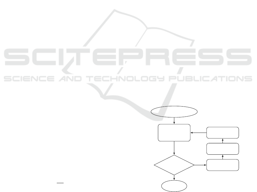
domly modifying solutions. The ﬂowchart of a typ-

ical GA is illustrated in ﬁgure 1. GA are well known

for parameter tuning but have also been extended to

perform structure optimization (Koza, 1992), an ap-

proach called genetic programming.

Initialization

Fitness

Evaluation

Converged?

Selection

Crossover

Mutation

Finish

Yes

Figure 1: Flowchart of a genetic algorithm.

Grammatical evolution (Ryan et al., 1998), a vari-

ation of GP, is based on the idea to deﬁne a gram-

mar in Backus-Naur form (BNF) (Backus, 1959; Naur

et al., 1969) to parse an integer string into an exe-

cutable program. This works by interpreting a string

Nonlinear Control Structure Design using Grammatical Evolution and Lyapunov Equation based Optimization

of integer numbers as a programming language. The

GE algorithm compiles this language using a gram-

mar in BNF. The generated program, which in many

applications is just a mathematical formula, can then

be evaluated. The result of this evaluation is rated by

a user-deﬁned metric, which serves as a ﬁtness value

for the corresponding individual. A grammar in BNF

can be described by the following deﬁnition.

Deﬁnition 6. A context free grammar is the 4-tuple

G = (N ,Σ, P,S) where N is the ﬁnite set of non-

terminals, Σ the ﬁnite set of terminals with N ∩Σ =

S ∈ N the start symbol. The vocabulary of G is V =

N ∪ Σ, which gives the ﬁnite set of production rules

as P ⊂ (V

∗

\ Σ

∗

) × V , each of the form N → V

∗

Here, ∗ denotes the Kleene star operator. Exam-

ple 1 shows, how this concept can be used to translate

an integer vector into a mathematical expression.

Example 1. We choose an example grammar G

like in deﬁnition 6 as N = {hei,hopi,hvi,hci},

Σ = {+, −,x, 1}, S = hei and P = {hei

→

hopi(hei,hei),hei

→ hvi,hei

→ hci,hopi

→ +,hopi

→

−,hvi

→ x,hci

→ 1}.

Consider an example individual, arbitrarily cho-

sen as i



6 4 1 2 5 2



. Dispatching the

current rule r

is done using the modulo operator as

GE,k

mod p where i

GE,k

is called the k-th codon of i

and p is the number of available rules from the cur-

rent non-terminal. This example starts with S = hei.

Since hei can be expanded by the three rules r

, r

, in the ﬁrst step, p = 3. Modulo dispatch selects

the ﬁrst rule since i

GE,1

mod p = 6 mod 3 = 0. The

translation process is then continued by unfolding all

nonterminals from left to right as shown in table 1.

Table 1: Parsing process on i

using G.

GE,k

p i

GE,k

mod p Rule Expression

- - - S hei

6 3 0 r

hopi(hei, hei)

4 2 0 r

+(hei, hei)

1 3 1 r

+(hvi, hei)

2 1 0 r

+(x, hei)

5 3 2 r

+(x, hci)

2 1 0 r

+(x, 1)

This procedure shows that the example individ-

ual represents the expression x + 1. If the mapping

is not ﬁnished yet but ran out of codons, the wrapping

technique is used, starting from the beginning of i

To avoid inﬁnite loops, a maximum wrapping count

is deﬁned. After exceeding this count, all recursive

rules are eliminated from P (in example 1 that would

be r

), such that the parsing is guaranteed to terminate

in a ﬁnite number of steps.

3 METHODS

3.1 Linear Performance Measures

For applicability and interpretability it is desirable to

deﬁne performance criteria from linear control theory

for the synthesized controllers. Therefore, we use Ja-

cobian linearization of the closed loop system about

the equilibrium x

∗

with δx = x − x

∗

. An approxima-

tion of the system dynamics by linearization is then

given by

δ ˙x =

∂ f

∂x



x=x

∗

δx = A

δx . (9)

The ﬁrst step is therefore to insert the GE-

generated control law into (8) and perform the above

linearization. Afterwards, methods from linear con-

trol theory can be applied as performance measures.

In this work we use a common approach for pole

placement presented in (Ackermann et al., 2002),

where a suitable region Γ in the complex s-plane is

deﬁned,



s = σ + jω : σ ≤ −

max



, (10)



s = σ + jω :

+ ω

≤ ω

max



, (11)



s = σ + jω : |ω| ≤

1 − ζ

min

|σ|



, (12)

Γ = Γ

∩ Γ

. (13)

Here, ζ

min

speciﬁes the minimum damping of the

system, T

max

the maximum time constant and ω

max

the maximum frequency of the linearized system

from (9). The area spanned by this deﬁnition is a cir-

cular sector with “cropped top”, an example is shown

in ﬁgure 2.

−6

−4 −2 0

−2

Real axis [s

−1

]

Imaginary axis [s

−1

]

Figure 2: Example Γ-region (grey) for pole placement.

To assign a ﬁtness value to a given controller, the

centroid of this region can be used. We propose the

ICINCO 2018 - 15th International Conference on Informatics in Control, Automation and Robotics

following analytic formula for the centroid of the Γ-

region from ﬁgure 2.

Proposition 1. The centroid s

= σ

+ jω

of the

stability area Γ spanned in the complex s-plane by

equation (13) as a function of the design parameters

min

, T

max

and ω

max

with ζ

min

∈ (0,1], T

max

> 0 and

max

> 1/T

max

is given by

= 0, σ







+ M

+ A

, ∆ > 0 (14a)

, ∆ ≤ 0 (14b)

where

∆ = ω

max

min

−

max

, (15)

max



2α − sin(2α)



, (16)

= −

max

sin

(α), (17)

1 − ζ

min

(ω

max

cos

(α)T

max

− 1)

2ζ

min

max

, (18)

−

1 − ζ

min

(ω

max

cos

(α)T

max

− 1)

3ζ

min

max

(19)

and

α =











arctan



1 − ζ

min



, ∆ > 0 (20a)

arccos



max



, ∆ ≤ 0. (20b)

Proof. Because of the symmetry of the Γ-region, ω

has to be 0. It is sufﬁcient to examine the curve above

the real axis. For the real part of the Γ-centroid, two

cases have to be considered.

Case 1. If ∆ ≤ 0, the Γ-region reduces to a circular

segment. Then σ

is given by M

, the known stan-

dard formula for the centroid of a circular segment.

Case 2. If ∆ > 0, σ

can be derived by calculating the

centroids of the circular segment and the remaining

quadrilateral. The centroid and the upper half of the

area of the circular segment are known as

C,1

= −

4ω

max

sin

(α)

3(2α − sin (2α))

, (21)

max

(2α − sin (2α)). (22)

The area and momentum of the upper half of the

quadrilateral can be computed using integration

= −

1 − ζ

min

−1/T

max

−ω

max

cos(α)

σdσ , (23)

= −

1 − ζ

min

−1/T

max

−ω

max

cos(α)

dσ , (24)

which then, with the relation σ

C,i

= M

, yields

the above result for the composite centroid of the Γ-

region.

Now we can deﬁne a ﬁtness measure for the GE

algorithm as follows.

Deﬁnition 7. Given the eigenvalues λ

from the sys-

tem matrix A

of a linearized system (9) and a Γ-

region deﬁned by the triple (T

max

,ζ

min

,ω

max

) the ﬁrst

part of the total ﬁtness value is given by

linear

= 1 +

∑

i=1



||λ

− s

, λ

/∈ Γ (25a)

0, λ

∈ Γ. (25b)

Remark 2. The value of φ

linear

describes the mean

deviation of the eigenvalues of A

not contained in Γ

from the geometrical mean (the centroid) of Γ. Note

that this only makes sense because Γ is convex and

connected. Otherwise the centroid is not guaranteed

to lie within the speciﬁed region.

Remark 3. In principle, different Γ-regions to the

proposed could be used. The advantage of this re-

gion however, is that it is widely used, compare (Ack-

ermann et al., 2002) or (Chilali and Gahinet, 1996),

can be parameterized by three meaningful values and

is both convex and connected, see remark 2.

Next, we want the controller not only to place the

poles of the linearized closed loop system (9) in the

Γ-region (13), but also to obtain a guaranteed domain

of attraction, which is as large as possible. We con-

tinue by stating this requirement as an optimization

problem and then propose a formulation compatible

to a GE algorithm, in order to make it computation-

ally tractable.

3.2 Domain of Attraction Estimation

To obtain an estimate for the stability region of the

synthesized controller, we use the fact that a subset of

the DoA (7), Ω

⊆ D(0) can be computed using

Ω

= {x ∈ R

: V (x) ≤ c}, (26)

with c ∈ R

, as long as V (x) fulﬁlls the Lyapunov

conditions from deﬁnition 4 on Ω

. The task of ﬁnd-

ing a controller that maximizes the domain of attrac-

tion and satisﬁes the constraints deﬁned in section 3.1

Nonlinear Control Structure Design using Grammatical Evolution and Lyapunov Equation based Optimization

can then be stated as the constrained, bilevel opti-

mization problem

maximize

u ∈ U(G)

L(Ω



) (27a)

subject to Ω



= {x ∈ R

: V (x) ≤ c



}, (27b)



= minimize

x ∈ R

6=0

V (x)

subject to

V (x) = 0,

(27c)

(27d)

) ∈ Γ ∀ i ∈ {1,. .. ,n} , (27e)

P + PA

+ Q = 0 , (27f)

P = P

 0, (27g)

V (x) = x

Px , (27h)

(x)| ≤ u

j,max

∀ j ∈ {1,. .. ,m} . (27i)

Here, L(Ω



) denotes the Lebesgue-measure of Ω



which can be interpreted as the maximum volume of

the estimated domain of attraction (26) for a given

u(x). Furthermore, U (G) is the function space of con-

trol laws u(x), that can be generated by a user-deﬁned

grammar G, speciﬁed in deﬁnition 6. Following, u

max

is the actuator limit, λ

) the i-th eigenvalue of A

(9) and Γ the region for pole placement (13). Equa-

tions (27c) and (27d) describe the standard optimiza-

tion problem of ﬁnding the largest level curve of V (x)

where

V (x)  0, for example discussed in (Saleme

et al., 2011). In the proposed setup, this is only one

constraint of the outer optimization problem (27a),

(27b) of ﬁnding a suitable control law u(x). Con-

straint (27e) ensures that the poles of the linearized

system (9) are placed in the Γ-region (13), while (27i)

limits control effort.

In order to produce correct results, it is necessary

that V (x)  0, which can be difﬁcult to test numer-

ically for arbitrary V (x). Therefore we use the so-

lution P of the Lyapunov equation, given Q  0, of

the linearized closed loop system (9) to construct a

symbolic representation of V (x) (27f), (27g), (27h).

In this work we choose Q as the identity matrix. Now

we perform a Monte Carlo sampling on V (x) and

V (x)

within a region of interest of the state space X

⊂ R

The time derivative

V (x) is calculated for the nonlin-

ear system symbolically by automatic differentiation.

The DoA is estimated using algorithm 1, which is a

modiﬁed version of the algorithm presented in (Na-

jaﬁ et al., 2016): We store the samples V (x

) in a list

L (line 5), which is used to estimate the DoA (lines

8-11). This algorithm is used to solve the inner opti-

mization problem (27c), (27d).

The proportion k/N is then a normalized approx-

imation of the size of the domain of attraction on the

sample set by Monte Carlo integration and gives the

ﬁnal ﬁtness measure to be minimized by the GE algo-

Algorithm 1: Domain of attraction estimation.

1: procedure DOASIZE(V (x),

V (x),X

,N)

2: Initialization: c ← ∞, k ← 0, L ←

3: for i ← 1 to N do

4: Pick random state x

∈ X

5: L ← (L,V (x

))  Store V (x

) in a list L

6: if V (x

) < c and

V (x

) ≥ 0 then

7: c ← V (x

)

8: for i ← 1 to N do  Estimate the DoA size

9: if L

< c then  L

is the i-th element of L

10: k ← k + 1

11: return k/N

rithm, which includes (27a)-(27h),

φ =



linear

, φ

linear

> 1 (28a)

1 − k/N , φ

linear

= 1 . (28b)

Additionally, we apply a smooth, symmetric satura-

tion with |u

(x)| ≤ u

j,max

(x) as shown in (Graichen

et al., 2010) to account for (27i). The function

j,sat

= u

j,max

−

j,max

1 + exp(2u

j,max

)

(29)

approximates a “hard” saturation, keeping u

sat

and

therefore the CLF differentiable.

Remark 4. While most methods cited in section 1 for

evaluating the quality of a Lyapunov function within

an EA framework for Lyapunov function synthesis use

some kind of sampling, most only count the propor-

tion of the samples that satisfy conditions in defnition

4. However, this measure is not very robust like the

example V (x

) = x

demonstrates. Since with ran-

dom samples, it is practically impossible to hit a value

on the zero line x

= 0, the algorithm will not detect

positive semi-deﬁniteness of V (x

). This however

is crucial for stability analysis since V (x

)  0 im-

plies that no conclusion about stability can be drawn.

Remark 5. Explicitly sampling on the axis x

= 0 us-

ing grid based techniques does not address the prob-

lem either as the example V (x

) = (sin(β)x

cos(β)x

)

with some β ∈ (−π/2,π/2) \ {0} shows.

We therefore expect a more robust measure using the

proposed method, since V (x), generated as a solution

to (27f), is automatically positive deﬁnite. If (27f) is

not solvable for some generated controller, it is as-

signed the worst possible ﬁtness, φ = ∞.

In the following section, we use a GE algorithm

to solve the optimization problem (27a)-(27i) for two

nonlinear benchmark systems in order to show the ef-

ﬁciency of the proposed method.

ICINCO 2018 - 15th International Conference on Informatics in Control, Automation and Robotics

4 EXPERIMENTS

4.1 Metrics and Setup

Table 2 shows the parameters of the GE algorithm.

Table 2: Grammatical evolution setup.

Parameter Value

Population size 100

Number of generations 5000

Mutation rate 0.05

Initial genome length ∼ U{10,20}

Initial genome values ∼ U{0,20}

Max. wrapping count 5

Max. tree depth 15

Selection Rank selection

Crossover Cut and splice

Mutation Uniform multi-point

Elitism rate 0.1

Selection pressure 1.5

Monte Carlo sample size 5000

The grammar G = (N ,Σ,P , S) used for the opti-

mization was chosen as

S = hei, (30)

N = {hei,hopi,hf i,hvi,hci}, (31)

Σ = {+,−, ×,/, sin,cos, arctan,x

,..., x

,C} , (32)

with the following mapping, denoted in BNF syntax,

by the production rules P ,

hei ::= hopi(hei, hei) | hf i(hei) | hvi | hci (33a)

hopi ::= + | − | × | / (33b)

hf i ::= sin | cos | arctan (33c)

hvi ::= x

| ... | x

(33d)

hci ::= C . (33e)

Here, C represents 10000 randomly generated con-

stants, drawn from a continuous uniform distribution

∼ U(−10,10). This provides a variety of different

constants for the GE algorithm, such that parameters

of the control law can be ﬁne-tuned.

4.2 Nonlinear Oscillator Example

We validate the proposed method on two different test

systems. The ﬁrst example is adopted from (Doyle

et al., 1996), describing a two dimensional oscillator

with highly nonlinear dynamics,

˙x

= x

(34)

˙x

= exp(x

)



cos(x

)sin(x

) − 2x

+ u



, (35)

with x

∈ [−4,4], x

∈ [−4,4]. Additionally we intro-

duce the constraint that u ∈ [−5,5]. The parameters

for the Γ-region were deﬁned as T

max

= 1 s, ζ

min

= 0.7

and ω

max

= 5 s

−1

. After several iterations, the GE

algorithm produces the following control law of non

obvious structure

= −3x

+ 2x

+ (x

− 2)x

, (36)

with the associated Lyapunov function

V (x) = 1.5x

+ 0.5x

+ x

. (37)

The eigenvalues of the closed loop system are both lo-

cated at (−1,0), satisfying the speciﬁed requirements

on the linearization of the system. We now use Jaco-

bian linearization (JL) of the uncontrolled, saturated

system and pole placement to generate a linear con-

troller with the same eigenvalues, given by

= −2x

. (38)

Notice that both controllers (36) and (38) have the

same linearized closed loop eigenvalues and therefore

the same quadratic Lyapunov function (37) according

to equation (27f). While their performance is there-

fore locally equivalent, it differs when getting farther

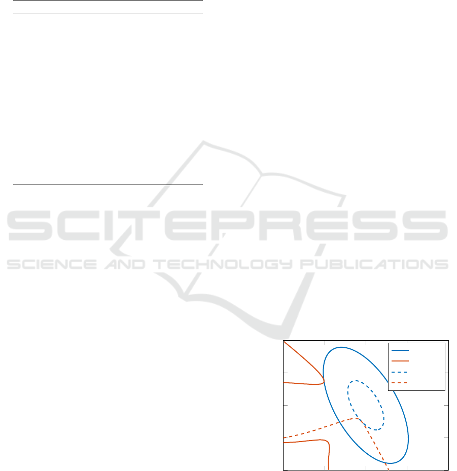
from the equilibrium. Figure 3 shows the estimated

domain of attraction for the GE controller (solid, blue)

and the linear controller (dashed, blue). The orange

lines indicate the level sets, where

V (x) = 0 for the

GE controller (solid, orange) and the linear controller

(dashed, orange). The GE controller shows a guaran-

teed DoA larger by a factor of 4.57 compared to the

linear controller. This estimate was computed using

algorithm 1 with a sample size of N = 10

. Notice,

that for the optimization itself, a signiﬁcantly smaller

sample size, namely N = 5000, as given in table 2,

was sufﬁcient to achieve this result.

−2 −1 0 1 2

−2

−1

GE DoA

V = 0

JL DoA

V = 0

Figure 3: Comparison of domains of attraction.

One single optimization run on this example took

approximately 30 seconds on a 2.8 GHz CPU, with

Nonlinear Control Structure Design using Grammatical Evolution and Lyapunov Equation based Optimization

the algorithm implemented in C++, using the options

from table 2. Out of 100 different, randomly initial-

ized optimization runs, each run produced a controller

that satisﬁed the linear requirements. Also, the associ-

ated Lyapunov function guaranteed stability in an area

of the state space approximately of the size shown in

ﬁgure 3 within ±5% deviation.

4.3 Anti-lock Braking Example

Additionally, we test the proposed method on a non-

linear anti-lock braking system (ABS) with longitu-

dinal vehicle dynamics using a quarter car model.

This model serves as another benchmark problem to

demonstrate the method. The system equations are

ω = −rF

− T

sign(ω) (39)

m ˙v = F

− F

. (40)

For details see for example (Petersen et al., 2001).

Here, ω is the angular velocity of the wheel, v the

longitudinal velocity of the vehicle and T

the brake

torque. Further, F

is the tire friction force, which

can be computed by the Pacejka tire model (Pacejka,

2005) as shown in (41) and F

the aerodynamic drag

force (42), given by

(λ,µ) = µ mg sin



arctan







, (41)

(v) =

ρA

v|v|, (42)

with λ, the longitudinal wheel slip deﬁned as

λ =

ωr − v

max(|ω|r,|v|)

. (43)

The friction coefﬁcient between tire and road is µ ∈

(0,1]. The other parameters are listed in table 3.

Table 3: Vehicle model parameters.

Name Description Value Unit

m Quarter car mass 450 kg

J Wheel moment of inertia 3 kgm

r Wheel radius 0.33 m

ρ Air density 1.1 kgm

−3

Vehicle front surface 2.4 m

Aerodynamic drag coef. 0.3 −

g Gravitational constant 9.81 ms

−2

Tire model slope coef. 10 −

Tire model shape coef. 1.3 −

act

Actuator time constant 0.025 s

Since the dynamics of the vehicle velocity evolve

signiﬁcantly slower than the angular wheel velocity,

it is common to assume ˙v ≈ 0. For the braking case,

the slip dynamics can be derived, compare (Petersen

et al., 2001). The state vector includes the tire slip

error x

= λ − λ

set

, its integral x

λ − λ

set

dτ and

actuator dynamics x

as x =





. The state

equations of the augmented error dynamics including

actuator dynamics are given as

˙x

= −



− u

max

+ u

∗

)



−



1 − λ



, (44)

˙x

= x

, (45)

˙x

act



u − x



, (46)

with λ = λ

set

= 0 and u

∗

required for shifting

the equilibrium of the system to the origin given as

∗

= F

(λ

set

,µ)

− J (λ

set

− 1)

max

r m

. (47)

The limit for the input is |u| ≤ 3000Nm = u

max

. The

region in the state space is deﬁned as x

∈ [−1,1],

∈ [−0.2,0.2], x

∈ [−1,1], the parameters for the Γ-

region as T

max

= 0.1s, ζ

min

= 0.4 and ω

max

= 30 s

−1

For the optimization we set

set

= 0,λ

set

= 0.5,µ =

0.2 and v = 50 km/h. After several iterations, the GE

algorithm produces the following control law of non

obvious structure

= −x

− 10.158x

+ x

arctan(ψ

), (48)

= x

− x

+ ψ

, (49)

= arctan(x

+ 11.16x

), (50)

= ψ

+ 11.16x

− 11.16). (51)

The Lyapunov function associated to system (46) with

controller (48) saturated by (29) is derived to

V (x) = x

Px = x





0.0869 0.4663 0.0247

0.4663 9.9604 0.0012

0.0247 0.0012 0.0271





x .

(52)

The eigenvalues of the closed loop system are located

at (−11.13,±20.68) and (−17.51,0), matching the

speciﬁed requirements. We now use Jacobian lin-

earization of (48) to generate a linear PI controller,

= −x

− 10.158x

. (53)

Notice that as in the previous example, both con-

trollers (48) and (53) have the same linearized closed

loop eigenvalues and therefore the same quadratic

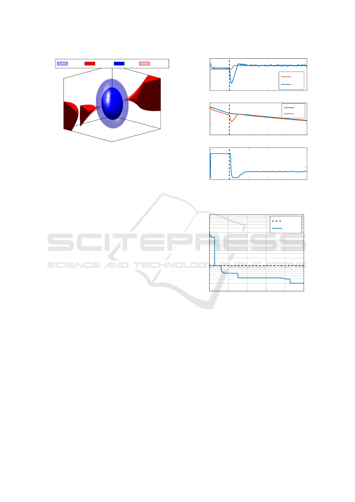
Lyapunov function. Figure 4 shows the DoA esti-

mates of the two methods on system (46).

The GE controller shows a DoA that is approxi-

mately 3.55 times larger than that of the PI controller.

This estimate was obtained using algorithm 1 with

a sample size of N = 10

. The nonlinearity in the

ICINCO 2018 - 15th International Conference on Informatics in Control, Automation and Robotics

−1

−0.1

0.1

−2

GE DoA GE

V ≥ 0 PI DoA PI

V ≥ 0

Figure 4: Comparison of domains of attraction.

control law (48) seems to be beneﬁcial for increas-

ing the guaranteed DoA in this case. Additionally,

we evaluate the nonlinear controller on the original

system (40). For the simulation, the controller (48)

is discretized with a sample time of 10 ms and acts

as a limiter for the brake force commanded by the

driver. The integrator state x

is fed back with anti-

windup. Furthermore, we add Gaussian white noise

with a signal-to-noise ratio of 50 dB to both ω and v

in order to simulate measurement noise. Communi-

cation delay is modeled with a time delay of 10 ms

for both the actuator and the sensors. The simulation

starts at v = 130 km/h and λ = 0 on dry asphalt with

µ = 1. The driver starts braking at t = 0 with 40%

braking force. At t = 1 s, the friction coefﬁcient of

the road drops to µ = 0.2 (snow). Therefore, the set-

point is changed to λ

set

= −3%. The controller gets

activated at t = 1.02 s, 20 ms after the event at t = 1 s.

Figure 5 shows the wheel slip λ as well as λ

set

, v, ω

and the control signal T

. The controller (48) iden-

tiﬁed by the GE algorithm successfully stabilizes the

nonlinear wheel dynamics. The wheel slip reaches

a peak value of ≈ 40%. The controller prevents the

wheels from decelerating further and therefore pre-

vents locking of the wheels.

One optimization run took again approximately

30 seconds on average. Figure 6 shows an example

error evolution of the best individual during one op-

timization run. It can be seen there that the linear

requirements are fulﬁlled at generation 281, where

φ ≤ 1 according to (28a) and (28b). At this point,

the constraints (27e)-(27i) are satisﬁed, as the poles

of the linearized closed loop system are located in the

speciﬁed Γ-region. Therefore, the Lyapunov equa-

tion (27f)-(27g) is guaranteed to have a unique so-

lution and a positive deﬁnite V (x) can be generated.

From thereon, the size of the guaranteed domain of at-

traction is increased over the subsequent generations.

0 1 2 3 4

−40

−20

Wheel slip [%]

set

0 1 2 3 4

100

150

Velocity [km/h]

ωr

0 1 2 3 4

500

1,000

1,500

Time [s]

[Nm]

Figure 5: Simulation of the tire slip controller (48).

0 1,000 2,000 3,000 4,000

5,000

−1

Generation

Fitness φ

φ = 1

Best φ

Figure 6: Example error evolution during the optimization.

Again, we evaluated the method for 100 different,

randomly initialized optimization runs, using the pa-

rameters from table 2 for the GE algorithm. As for

the nonlinear oscillator benchmark system from sec-

tion 4.2, each run produced a controller that placed the

poles of the linearized closed loop system in the de-

sired Γ-region. This was despite the fact that all runs

started with all, or at least some of the poles being

located outside of the Γ-region. The distance of the

poles to the centroid of the Γ-region was successfully

used as a performance measure for pole placement.

The average ﬁtness achieved over all 100 optimiza-

tion runs was 0.4419 with a variance of 0.0662.

Nonlinear Control Structure Design using Grammatical Evolution and Lyapunov Equation based Optimization

5 CONCLUSION

A new method for controller synthesis based on gram-

matical evolution has been proposed. We derived an

explicit formula for the centroid of the considered sta-

bility region used for pole placement and integrated it

into a GE optimization algorithm. Additionally, the

GE algorithm was extended to maximize the guaran-

teed domain of attraction by using Monte Carlo inte-

gration in order to solve a bilevel optimization prob-

lem. On the considered nonlinear oscillator system

and the ABS control system, the method showed con-

vincing performance for maximizing the guaranteed

domain of attraction while satisfying the speciﬁed

constraints. For the ABS system, the generated con-

troller was validated by simulation. One limitation of

the presented approach is that it is computationally

expensive such that it cannot be applied as an online

optimization method.

Future work can extend the proposed approach in

different directions. One possibility is to include fur-

ther linear performance measures into the optimiza-

tion process. For example, the parameter space ap-

proach (Ackermann et al., 2002) provides measures

to ensure robustness of the controller with respect to

uncertain parameters for the linearized system. Also,

different Γ-regions than the proposed one might be

used for the optimization. Further, it would be in-

teresting to evaluate more algorithms for estimating

the domain of attraction, for example using a sam-

pling algorithm with memory as proposed in (Najaﬁ

et al., 2016). Also, the MIMO (multi-input, multi-

output) case could be investigated. Finally, one could

remove the assumption of a quadratic Lyapunov func-

tion and let the GE algorithm search for the structure

of both the Lyapunov function and the control laws at

the same time. However, as mentioned in remarks

4 and 5, ensuring positive deﬁniteness in this gen-

eral setup might be challenging. Future work could

therefore focus on creating algorithms that can reli-

ably detect positive semi-deﬁniteness of general, non-

quadratic Lyapunov functions.

The presented approach is applicable for nonlinear

control synthesis for a large range of nonlinear sys-

tems with different types of nonlinearities. Input con-

straints and performance speciﬁcations adopted from

linear control theory can be incorporated into the con-

trol design process. In general, the system order is not

restricted. The method presents a nonlinear control

structure design tool which is applicable to a variety

of practical applications. Results suggest that reason-

able stability guarantees are achieved with the combi-

nation of structural control law optimization and do-

main of attraction maximization.

REFERENCES

Ackermann, J., Blue, P., B

unte, T., G

uvenc, L., Kaes-

bauer, D., Kordt, M., Muhler, M., and Odenthal, D.

(2002). Robust control: the parameter space ap-

proach. Springer Science & Business Media.

Backus, J. W. (1959). The syntax and semantics of the pro-

posed international algebraic language of the Zurich

ACM-GAMM conference. Proceedings of the Inter-

national Conference on Information Processing.

Banks, C. (2002). Searching for Lyapunov func-

tions using genetic programming. Virginia Poly-

tech Institute and State University, Blacksburg,

Virginia. Available online (last visit 24/05/2018):

http://www.aerojockey.com/ﬁles/lyapunovgp.pdf.

Bartels, R. H. and Stewart, G. (1972). Solution of the matrix

equation AX +XB = C: Algorithm 432. Communica-

tions of the ACM, 15(9):820–826.

Chen, P. and Lu, Y.-Z. (2011). Automatic design of ro-

bust optimal controller for interval plants using ge-

netic programming and Kharitonov theorem. Interna-

tional Journal of Computational Intelligence Systems,

4(5):826–836.

Chen, Z., Mi, C. C., Xiong, R., Xu, J., and You, C.

(2014a). Energy management of a power-split plug-in

hybrid electric vehicle based on genetic algorithm and

quadratic programming. Journal of Power Sources,

248:416–426.

Chen, Z., Yuan, X., Ji, B., Wang, P., and Tian, H. (2014b).

Design of a fractional order PID controller for hy-

draulic turbine regulating system using chaotic non-

dominated sorting genetic algorithm II. Energy Con-

version and Management, 84:390–404.

Chilali, M. and Gahinet, P. (1996). H

∞

design with pole

placement constraints: an LMI approach. IEEE Trans-

actions on automatic control, 41(3):358–367.

Cupertino, F., Naso, D., Salvatore, L., and Turchiano, B.

(2002). Design of cascaded controllers for DC drives

using evolutionary algorithms. In Evolutionary Com-

putation, 2002. CEC’02. Proceedings of the 2002

Congress on, volume 2, pages 1255–1260. IEEE.

Doyle, J., Primbs, J. A., Shapiro, B., and Nevistic, V.

(1996). Nonlinear games: examples and counterex-

amples. In Decision and Control, 1996., Proceed-

ings of the 35th IEEE Conference on, volume 4, pages

3915–3920. IEEE.

Gholaminezhad, I., Jamali, A., and Assimi, H. (2014). Au-

tomated synthesis of optimal controller using multi-

objective genetic programming for two-mass-spring

system. In Robotics and Mechatronics (ICRoM), 2014

Second RSI/ISM International Conference on, pages

041–046. IEEE.

Giesl, P. and Hafstein, S. (2015). Review on computational

methods for Lyapunov functions. Discrete and Con-

tinuous Dynamical Systems, Series B, 20(8):2291–

2337.

Glover, F. W. and Kochenberger, G. A. (2006). Handbook of

metaheuristics, volume 57. Springer Science & Busi-

ness Media.

ICINCO 2018 - 15th International Conference on Informatics in Control, Automation and Robotics

Graichen, K., Kugi, A., Petit, N., and Chaplais, F. (2010).

Handling constraints in optimal control with satura-

tion functions and system extension. Systems & Con-

trol Letters, 59(11):671–679.

Grosman, B. and Lewin, D. R. (2005). Automatic gener-

ation of Lyapunov functions using genetic program-

ming. IFAC Proceedings Volumes, 38(1):75–80.

Haupt, R. L. and Haupt, S. E. (1998). Practical genetic

algorithms, volume 2. New York: Wiley.

Holland, J. H. (1975). Adaptation in natural and artiﬁcial

systems: an introductory analysis with applications to

biology, control, and artiﬁcial intelligence. University

of Michigan Press.

Hosen, M. A., Khosravi, A., Nahavandi, S., and Creighton,

D. (2015). Improving the quality of prediction inter-

vals through optimal aggregation. IEEE Transactions

on Industrial Electronics, 62(7):4420–4429.

Koza, J. R. (1992). Genetic programming: on the program-

ming of computers by means of natural selection, vol-

ume 1. MIT press.

Koza, J. R., Keane, M. A., Yu, J., Bennett, F. H., Myd-

lowec, W., and Stiffelman, O. (1999). Automatic syn-

thesis of both the topology and parameters for a robust

controller for a nonminimal phase plant and a three-

lag plant by means of genetic programming. In Deci-

sion and Control, 1999. Proceedings of the 38th IEEE

Conference on, volume 5, pages 5292–5300. IEEE.

Koza, J. R., Keane, M. A., Yu, J., Mydlowec, W., and Ben-

nett, F. H. (2000). Automatic synthesis of both the

topology and parameters for a controller for a three-

lag plant with a ﬁve-second delay using genetic pro-

gramming. In Workshops on Real-World Applica-

tions of Evolutionary Computation, pages 168–177.

Springer.

Lyapunov, A. M. (1992). The general problem of the sta-

bility of motion. International Journal of Control,

55(3):531–534.

McGough, J. S., Christianson, A. W., and Hoover, R. C.

(2010). Symbolic computation of Lyapunov functions

using evolutionary algorithms. In Proceedings of the

12th IASTED International Conference, volume 15,

pages 508–515.

Mirafzal, S. H., Khorasani, A. M., and Ghasemi, A. H.

(2016). Optimizing time delay feedback for active

vibration control of a cantilever beam using a ge-

netic algorithm. Journal of Vibration and Control,

22(19):4047–4061.

Najaﬁ, E., Babu

ska, R., and Lopes, G. A. (2016). A fast

sampling method for estimating the domain of attrac-

tion. Nonlinear Dynamics, 86(2):823–834.

Naur, P., Backus, J. W., Bauer, F. L., Green, J., Katz, C.,

McCarthy, J., and Perlis, A. J. (1969). Revised report

on the algorithmic language Algol 60. Springer.

Pacejka, H. (2005). Tyre and vehicle dynamics. Butter-

worth-Heinemann, Oxford, 2 edition.

Petersen, I., Johansen, T. A., Kalkkuhl, J., and L

udemann,

J. (2001). Wheel slip control in ABS brakes using

gain scheduled constrained LQR. In European Con-

trol Conference (ECC), pages 606–611. IEEE.

Poli, R., Langdon, W. B., and McPhee, N. F. (2008). A

ﬁeld guide to genetic programming. Published via

http://lulu.com and freely available online (last visit

24/05/2018) http://www.gp-ﬁeld-guide.org.uk. (With

contributions by J. R. Koza).

Prajna, S., Papachristodoulou, A., and Parrilo, P. A. (2002).

Introducing SOSTOOLS: A general purpose sum of

squares programming solver. In Decision and Control,

2002, Proceedings of the 41st IEEE Conference on,

volume 1, pages 741–746. IEEE.

Precup, R.-E., Sabau, M.-C., and Petriu, E. M. (2015).

Nature-inspired optimal tuning of input membership

functions of Takagi-Sugeno-Kang fuzzy models for

anti-lock braking systems. Applied Soft Computing,

27:575–589.

Reichensd

orfer, E., Odenthal, D., and Wollherr, D. (2017).

Grammatical evolution of robust controller structures

using Wilson scoring and criticality ranking. In Eu-

ropean Conference on Genetic Programming, pages

194–209. Springer.

Ryan, C., Collins, J., and Neill, M. O. (1998). Grammati-

cal evolution: evolving programs for an arbitrary lan-

guage. In European Conference on Genetic Program-

ming, pages 83–96. Springer.

Saadat, J., Moallem, P., and Kooﬁgar, H. (2017). Training

echo state neural network using harmony search algo-

rithm. International Journal of Artiﬁcial Intelligence,

15(1):163–179.

Saleme, A., Tibken, B., Warthenpfuhl, S. A., and Selbach,

C. (2011). Estimation of the domain of attraction for

non-polynomial systems: A novel method. IFAC Pro-

ceedings Volumes, 44(1):10976–10981.

Shimooka, H. and Fujimoto, Y. (2000). Generating robust

control equations with genetic programming for con-

trol of a rolling inverted pendulum. In Proceedings of

the 2nd Annual Conference on Genetic and Evolution-

ary Computation, pages 491–495. Morgan Kaufmann

Publishers Inc.

Singh, R., Kuchhal, P., Choudhury, S., and Gehlot, A.

(2015). Implementation and evaluation of heating sys-

tem using PID with genetic algorithm. Indian Journal

of Science and Technology, 8(5):413.

Sontag, E. D. (1983). A Lyapunov-like characterization of

asymptotic controllability. SIAM Journal on Control

and Optimization, 21(3):462–471.

Tsuzuki, T., Kuwada, K., and Yamashita, Y. (2006). Search-

ing for control Lyapunov-Morse functions using ge-

netic programming for global asymptotic stabilization

of nonlinear systems. In Proceedings of the 45th IEEE

Conference on Decision and Control, pages 5114–

5119. IEEE.

Verdier, C. and Mazo Jr, M. (2017). Formal controller syn-

thesis via genetic programming. IFAC-PapersOnLine,

50(1):7205–7210.

Vrkalovic, S., Teban, T.-A., and Borlea, I.-D. (2017). Stable

Takagi-Sugeno fuzzy control designed by optimiza-

tion. Int. J. Artif. Intell, 15:17–29.

Zhou, K., Doyle, J. C., Glover, K., et al. (1996). Robust and

optimal control, volume 40. Prentice hall New Jersey.

Nonlinear Control Structure Design using Grammatical Evolution and Lyapunov Equation based Optimization