A Fault-Tolerant Sensor Reconciliation Scheme

based on Self-Tuning LPV Observers

Hamid Behzad

, Alessandro Casavola

, Francesco Tedesco

Mohammad Ali Sadrnia

and Gianfranco Gagliardi

Shahrood University of Technology, Iran

University of Calabria, DIMES, Italy

Keywords:

Sensor Reconciliation, Fault Estimation, LPV Luenberger Observer.

Abstract:

This paper presents a fault-tolerant sensor reconciliation scheme for systems equipped with a redundant num-

ber of possibly faulty ”physical” sensors. The reconciliator is in charge to discover on-line, at each time

instant, the faulty physical sensors, if any, and exclude their measures from the generation of the ”virtual”

sensors, which, on the contrary, are supposed to be always healthy and suitably usable for control purposes

without requiring the reconﬁguration of the nominal control law. Amongst many, the solution proposed here

is based on the use of a Linear Parameter Varying Luenberger Observers (LPV-LU) able to estimate both

state, bias fault and loss of effectiveness fault. Such information is used to self adapting the parameters of the

LPV representation. For simplicity, the sensor faults here considered are limited to variation of sensors’ gain

and offset values. The scheme is fully described and all of its properties investigated and proved. Finally, a

simulation example is reported in details to show the effectiveness of the scheme.

1 INTRODUCTION

The capability of control systems to detect faulty sen-

sors and recover in turn uncorrupted data has progres-

sively gained more relevance in the last two decades.

Traditional control schemes are usually designed by

assuming perfect working conditions of the sensors

to be used. However, in practice, sensors are subject

to faults and, in that case, may provide wrong infor-

mation about the system state, possibly degrading the

system performance or even causing instability (Mer-

rill et al., 1988; Samara et al., 2008). Therefore,

Fault-Tolerant Control (FTC) is an important area of

research in the safety critical systems domain.

One strategy to cope with this situation is to ﬁnd

a controller that assigns to the reconﬁgured closed-

loop system a similar behaviour with respect to the

nominal closed-loop system. A different strategy re-

lies on the fault hiding approach that tries to hide the

fault to the controller. In the latter approach the nom-

inal controller remains in the loop while the reconﬁg-

uration block re-routes the output signals around the

faulty component (Lunze and Richter, 2008). Such

an approach has been dealt with in (Steffen, 2005)

where a virtual sensor strategy has been proposed for

fault accommodation purposes. The disadvantage of

that method is that it is assumed that the sensor faults

have already been detected and estimated correctly.

The virtual sensors contribution to Active Fault Toler-

ant Control (AFTC) has been investigated in (Ponsart

et al., 2010). There, the case of multiplicative sen-

sor faults has not received any consideration. The vir-

tual sensor approach has been investigated in (Behzad

et al., 2016), for Sensor Reconciliation(SR) purposes.

This paper aims at presenting a general SR method

for discrete-time linear systems with redundant phys-

ical sensors possibly subject to loss of effectiveness

(gain) and offset (bias) faults. To this end, the pro-

posed scheme consists of two interconnected mod-

ules: (i) a polytopic Luenberger Observer (LU) ((Bara

et al., 2001)) in charge of estimating the current gain

sensor faults, the state of the system and possible bias

fault occurrences; (ii) a sensor reconciliation unit used

to reconcile sensor measures. The key idea used in

the proposed scheme is to consider the current gain

and bias sensor faults with the system states, as an

auxiliary state and consequently to design a polytopic

LPV-UIO observer capable to estimate the faults via

a speciﬁc Linear Matrix Inequality (LMI) procedure.

Differently from (Behzad et al., 2016), where the con-

Behzad, H., Casavola, A., Tedesco, F., Sadrnia, M. and Gagliardi, G.

A Fault-Tolerant Sensor Reconciliation Scheme based on Self-Tuning LPV Observers.

DOI: 10.5220/0006840501110118

In Proceedings of the 15th International Conference on Informatics in Control, Automation and Robotics (ICINCO 2018) - Volume 1, pages 111-118

ISBN: 978-989-758-321-6

111

vergence of the scheme was based on a persistence of

excitation assumption, here we propose a Luenberger

observer to jointly estimate the system state and fault

parameters in a single step in order to guarantee the

convergence of the whole scheme. Moreover, unlike

the approach of (Steffen, 2005), our setup is capable

of fault estimation along with fault accommodation.

The key difference of our approach with respect to

(Ponsart et al., 2010) is that both the multiplicative

and additive faults may be taken into consideration.

Properties of the proposed LPV-LU scheme are for-

mally proved and discussed. A ﬁnal numerical exam-

ple is reported to show the effectiveness of the pro-

posed strategy.

NOTATION

Let R denote the set of real numbers. A generic ball

in an Euclidean n-space R

is deﬁned as B

:= {x ∈

: |x|

≤ δ}. Finally, let kx(·)k denote the `

-norm

of a discrete-time signal {x(t)}

∞

−∞

(i.e. kx(·)k =

∑

∞

t=−∞

|x(t)|

Deﬁnition 1.1. (Cartesian Product) - For P ∈ R

and

Q ∈ R

being two polytopes of dimension p and q

respectively, their Cartesian Product is deﬁned as

P × Q = {(x,y) : x ∈ P ,y ∈ Q }

Deﬁnition 1.2. (Unit Simplex) - The Polytope S

{ξ ∈ R

|ξ

≥ 0, i = 1,...,l,

∑

i=1

= 1} is a k-

dimensional Unit Simplex.

Deﬁnition 1.3. (Convex hull) - For l matrices

∈ R

n×m

, i = 1, ..., l, their Convex Hull, de-

noted by Co{M

},i = 1, ..., l, is the polytope aris-

ing by all convex combinations of matrices M

i.e

{

∑

i=1

,[ρ

,...,ρ

]

∈ S

} with S

being a l-

dimensional unit simplex.

Deﬁnition 1.4. (Pontryagin Set Difference) - For

given sets A, E ⊂ R

, the set determined as A ∼ E :=

{a : a + e ∈ A,∀e ∈ E} is the Pontryagin Set Differ-

ence of A with respect to E.

2 PROBLEM FORMULATION

Let us consider a plant whose dynamics is described

by the following discrete-time state-space representa-

tion

(t + 1) = Ax

(t) + Bu(t) + Ev(t) (1)

y(t) = ∆



γ(t)



(t) + Fb(t) (2)

z(t) = H

(t) (3)

where A ∈ R

n×n

, B ∈ R

n×n

, E ∈ R

n×n

, C

∈ R

m×n

and

F ∈ R

m×q

are constant matrices. Moreover, x

(t) ∈

is the state vector assumed to be conﬁned in the

following set

:= {x

: x

≤ x

} (4)

Notice that the upper and lower bounds are re-

quired to describe the polytopic representation of the

output. This representation will be used to design a

LPV observer.

Moreover u(t) ∈ R

is a known input while v(t) ∈

is an unknown input. y(t) ∈ R

represents the

plant output provided by physical redundant sensors

possibly effected by both bias b(t) ∈ R

and loss of ef-

fectiveness faults, the latter being modeled by the gain

matrix ∆(γ) ∈ R

m×m

that, for simplicity, we assume

hereafter to have the following elementary structure:

∆(γ(t)) =







(t) 0 0

0 0 γ

(t)







(5)

Finally, z(t) ∈ R

, with r ≤ m, is deﬁned as the

virtual output of the system and represents the healthy

information we need to get from the plant for control

purposes regardless of any fault possibly occurring on

the physical sensors.

It is clear that in the absence of faults one would

have ∆(γ) = I

and b(t) = 0

. However, in the more

general case b(t) 6= 0

and ∆(γ) 6= I

, with γ conﬁned

in the generic polytope

Γ ⊆ {γ : 0

≤ γ ≤ 1

} (6)

For this reason, it is not convenient to evaluate

the signal z(t) as z(t) = H

y(t) because it would be

affected by possibly corrupted information brought

by y(t). However, because the state x

(t) is assumed

not directly measurable, z(t) cannot be evaluated as

simply as in (3), but a more sophisticated machinery

is required. This aspect motivates the design of the

Sensor Reconciliator unit before mentioned which

basically aims at addressing the following problem:

Sensor Reconciliaton Design Problem (SRDP-

Problem):

Given the system (1)-(3), compute, at each time

t ≥ 0 on the basis of the real output y(t) mea-

sures, a suitable estimate ˆz(t) of the virtual output

z(t) := H

(t), despite of the presence of both

fault occurrences, corrupting the vectory(t), and

disturbances v(t).

ICINCO 2018 - 15th International Conference on Informatics in Control, Automation and Robotics

112

Faulty

sensors

UIO unit

Reconciliator

Unit

Virtual Sensor

Figure 1: Virtual Sensor Architecture.

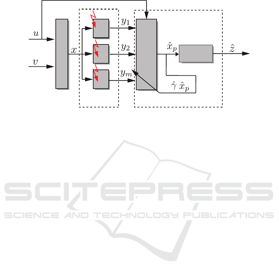
3 VIRTUAL SENSOR

ARCHITECTURE

The SRDP-Problem solution here proposed is based

on the evaluation of an estimate ˆx

(t) of the state x

(t)

that is exploited to compute the corresponding ap-

proximation ˆz(t) of z(t) through the following equa-

tion

ˆz(t) = H

ˆx

(t) (7)

Such an approach requires to face two crucial is-

sues: 1) How to estimate the fault occurrences cor-

rupting y(t)? 2) How to get a good estimation ˆx

(t)

in the presence of an unknown input v(t) and time-

varying sensor gains and bias?

The above mentioned questions are dealt with by

introducing the virtual sensor architecture depicted in

Fig. 1 that consists of two modules: a Luenberger

Observer (LO) unit which is the core of this scheme

and is designed to jointly compute current estimates

of the state x

(t) , the bias term b(t) and the effective-

ness matrix (5) parameters; a Reconciliator Unit that

simply performs the computation indicated in (7).

4 SENSOR FAULT AUGMENTED

MODEL

In order to design the Luenberger observer, the fol-

lowing augmented state is considered that includes

the bias fault b(t) and multiplicative fault γ(t) vector

among its components

x(t) =







(t)

b(t)

(t)







(8)

Notice that in order to describe the augmented

model, one has to assume that the multiplicative sen-

sor fault term γ(t), the bias term b(t) and the parame-

ters ∆γ(t) and ∆b(t) are bounded in the l

norm sense,

where

∆b(t) := b(t + 1) − b(t)

∆γ(t) := γ(t + 1) − γ(t)

In this way, the related augmented model can be de-

scribed as

x(t + 1) =

Ax(t) +

Bu(t) +

Ev(t)

F∆b(t) +

D∆γ(t)

¯y(t) =

γ(t),x

(t)

x(t) (9)

where

A =





A 0 0

0 I 0

0 0 I





B =









E =









F =









{γ(t),x

(t)}



4(γ(t))C

F 0

0 F diag(C

(t))



D =









(10)

5 LUENBERGER OBSERVER

In this section we describe the basic ingredients of the

proposed observer. Let us assume to be provided with

A Fault-Tolerant Sensor Reconciliation Scheme based on Self-Tuning LPV Observers

113

estimates

γ(t) of γ(t) and ˆx

(t) of x

(t) at each time

t. Then, a possible structure for an observer for the

model (9) is given by

ˆx(t + 1) =

A ˆx(t) +

Bu(t) +L



¯y(t) − ˆy(t)



ˆy(t) =

{

γ(t), ˆx

(t)}

ˆx(t) (11)

As a consequence, the one-step ahead evolution of

the state estimation error

e(t) := x(t) − ˆx(t) (12)

would take the following form

e(t + 1) =



A − L

γ(t), ˆx

(t)

{

γ(t), ˆx

(t)}



e(t) +

Ev(t)

F∆b(t) +

D∆γ(t) − L

γ(t), ˆx

(t)

d(t) (13)

with

d(t) :=



{γ(t),x

(t))}

−

{

γ(t), ˆx

(t)}



x(t)



A − L

{

γ(t), ˆx

(t)}

{

γ(t), ˆx

(t)}



were chosen as a sta-

ble matrix ∀γ ∈ Γ and ∀x

∈ X

, the state estimation

error would remain bounded whenever ∆b(t) and

∆γ(t) remain bounded as well. Hence, the state x(t)

of the system can be estimated.

Moving from these considerations, in order to de-

sign the Luenberger observer (11), it is is sufﬁcient

to determine a parameter varying gain L

γ,x

that ro-

bustly stabilizes the system (13) against all possible

occurrences of ∆b(t), ∆γ(t) and d(t). Such a problem

has been addressed in a signiﬁcant amount of works

in different contexts by exploiting well-known results

on robust control theory and LMI formalism. Specif-

ically, among many observer design approaches, it is

interesting to mention here (Heemels et al., 2010),

where the LPV gain is determined in the case of con-

stant output matrix. A similar approach has been con-

sidered in (Zhou et al., 2013), where a LMI based pro-

cedure has been proposed to compute a constant gain.

Here we design a discrete-time self-tuning LPV

observer where the time-varying parameter γ and the

state x

are not perfectly known. In particular, the

approach considers systems (13) characterized by a

structured uncertainty related to γ , x

and attempts to

determine a LPV gain that can be tuned on-line by ex-

ploiting an estimate

γ(t) and ˆx(t) of the true γ(t) and

x(t). In this respect, it is worth pointing out that we

assume hereafter to be provided by a polytopic em-

bedding approximation for matrix

{

γ(t), ˆx

(t)}

given

∑

i=1

(γ,x

)

, (14)

for a certain continuous functions ρ

: Γ ×X

∼ B

→

R of γ and x

and matrices

, i = 1, ..., l.

Now, we have all the ingredients to design a LPV

gain L

deﬁned as follows

∑

i=1

(γ,x)L

(15)

where the gains L

, i = 1, ..., l are properly chosen to

stabilize the observer with the estimation error subject

e(t + 1) = N

ρ(t)

e(t) + F

ρ(t)

w(t) (16)

with



A − L





F T

D −L



, w(t) :=







v(t)

∆b(t)

∆γ(t)

d(t)







(17)

In addition, those gains have to guarantee that for each

estimate

γ, ˆx

lies in the convex hull Co{

},i =

1,...,l. Moreover it is assumed that the signal w(t)

belong to `

space with a known bound ¯w on its `

norm, i.e.

kw(·)k ≤ ¯w (18)

Then the problem just stated translates into ﬁnding a

parameter-dependent gain such that difference equa-

tion (16) is stable for any arbitrary time variation of

the parameters

ρ(t) ∈ S

and such that, for any input

w(t) satisfying (18), the error e(t) is bounded as

||e(·)|| < σ||w(·)||, (19)

A convex optimization methodology to solve the

above stated design problem is provided in the next

Theorem 1.

Theorem 1. Assume a symmetric strictly positive def-

inite matrices P

and matrices G

and Y

, i = 1,...,l

exist such that the optimization problem

min

,µ

subject to

i j





+ G

− P

? P

− I 0

? ? µI





> 0, µ <

¯w

i = 1, ..., l, j = 1, ...,l

:= G

A −Y

(20)

ICINCO 2018 - 15th International Conference on Informatics in Control, Automation and Robotics

114

i jk





∗ P

+ P

− I 0

∗ ∗ µI





> 0

i = 1, ..., l − 1, j = 1, ..., l, k = i + 1,...,l

:= G

+ G

+ P

:= G

A + G

A −Y

−Y

:= G

+ G

(21)

has a solution. Then, the convergence of the observer

estimation error dynamically characterized by equa-

tion (16) is ensured, the guaranteed H

∞

performance

gain (19) given by

σ =

¯w

, µ

= minµ (22)

is achieved and

ρ(t) is ensured to vary into S

. More-

over, the observer gain vertices deﬁned in (15) are

given by

= G

−1

,i = 1,...,l (23)

and stabilize the observer for any arbitrary time vari-

ation of the parameter

ρ(t) in the polytope S

Proof : Consider the parameter-dependent Lya-

punov function



e(t)



= e

(t)P

ρ(t)

e(t) (24)

with

ρ(t)

∑

i=1

(t)P

= P

, i = 1, ..., l (25)

The related one-step ahead evolution of the Lyapunov

function on the observer error trajectory is given by



e(t + 1)



= e

(t + 1)P

ρ(t+1)

e(t + 1) (26)

where P

ρ(t+1)

can be written as

ρ(t)

∑

j=1

(t)P

= P

, j = 1,...,l (27)

Using (27), one can recast (26) into



e(t + 1)





ρ(t)

e(t) + F

ρ(t)

w(t)



ρ(t)



ρ(t)

e(t) + F

ρ(t)

w(t)



(28)

Then, the Lyapunov function increment derived

by (24) and (28) results to be given by

∆V (e(t)) = V (e(t + 1)) −V (e(t))

= e

(t)



ρ(t)

− P

ρ(t)



e(t)

+ 2e

(t)N

ρ(t)

w(t)

+ w

(t)F

ρ(t)

w(t) (29)

It is well-known that the stability of system with H

∞

guaranteed performance (19) is ensured if

∆V (e(t)) < −e

(t)e(t) + µw

(t)w(t), ∀t (30)

By replacing ∆V (e(t)) with the expression (29), one

is able to rewrite (30) as Γ

(t)UΓ(t) < 0 with Γ(t) :=



(t) w

(t)



and

U :=



? U



(31)

:= N

ρ(t)

− P(ρ(t)) + I

:= N

ρ(t)

, U

:= F

ρ(t)

− µI

Clearly, by imposing U < 0 it is possible to guarantee

(30) for all e(t) 6= 0 and w(t) 6= 0 by satisfying the

following inequality

ρ(t)

(ρ(t))P

ρ(t)

−1

ρ(t)



ρ(t)



−



ρ(t)

− I 0

0 µI



< 0

(32)

The latter, thanks to the use of a Schur’s comple-

ment argument, is equivalent to





ρ(t)

? P

ρ(t)

− I 0

? ? µI





> 0 (33)

that can be recast into

> 0 with M :=





ρ(t)

−1

ρ(t)

0 0

0 I 0

0 0 I





(34)

and, in turn, into





ρ(t)

−1

ρ(t)

? P

ρ(t)

− I 0

? ? µI





> 0 (35)

Using previously deﬁned matrices and considering

that ρ ∈ S

and

ρ ∈ S

, inequality (35) can be written

∑

i=1

(t)

∑

j=1

(t)Ξ

i j

l−1

∑

i=1

∑

k=i+1

(t)

∑

j=1

(t)Ξ

i jk

> 0

(36)

with Ξ

i j

deﬁned in (20) and Ξ

i jk

deﬁned in (21). For

more details please refer to (Heemels et al., 2010). 

A Fault-Tolerant Sensor Reconciliation Scheme based on Self-Tuning LPV Observers

115

0 1000 2000 3000 4000 5000 6000 7000

-150

-100

-50

100

150

Known Input

Time(Steps)

0 1000 2000 3000 4000 5000 6000 7000

100

Unknown Input

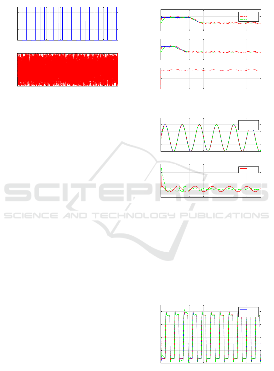
Figure 2: Known Input (up) and Unknown Input (down).

6 ILLUSTRATIVE EXAMPLE

In this section, the effectiveness of the proposed UIO-

SR scheme is investigated by considering the follow-

ing linear stable model

(t + 1) = Ax

(t) + Bu(t) + Ev(t)

y(t) = ∆(γ(t))C

(t) + Fb(t) (37)

where

A =



0.98806 0.0096049

−0.32754 0.93033



,B =



−0.0001

−0.0921



1 0

1 1

,E = 0.01 ×





F =

with γ assumed to be conﬁned within the polytope

Γ :=

γ : [γ

,γ

]

≤ γ ≤ [γ

,γ

]

,γ

= γ

0, γ

= 0.1, γ

= 1, i = 1,2,3.

The goal of this simulation is to verify the capa-

bility of the proposed method to correctly estimate

the ﬁrst component of x

(t) in (37) under faults that is

used as virtual output z(t) = H

(t) for the system.

Correspondingly, the following sensor reconciliation

matrix



0.5 0.5 0



(38)

results with the known input u(t) depicted in Figure

2 (up) and the unknown input v(t) supposed to be a

white noise with standard deviations equal to 10 (de-

picted in Figure 2 (down)). Moreover, the bias proﬁle

on the three available physical sensors is assumed to

change along the simulation time according to the

0 1000 2000 3000 4000 5000 6000 7000

-1

Gain Fault Estimation(∆

)

Real

LPV-UIO

LPV-LU

0 1000 2000 3000 4000 5000 6000 7000

-1

Time(Steps)

0 1000 2000 3000 4000 5000 6000 7000

0.5

Figure 3: Loss of effectiveness parameters.

0 1000 2000 3000 4000 5000 6000 7000

f(t)

-100

-50

100

150

Bias Fault Estimation

Real

LPV-UIO

LPV-LU

Time(Steps)

0 1000 2000 3000 4000 5000 6000 7000

f(t)

-10

Bias Fault Estimation Error

LPV-UIO

LPV-LU

Figure 4: Bias fault and its estimation.

following proﬁle

b(t) = 1 + 100sind(0.3t) (39)

and faults on the matrix effectiveness gain will affect

the ﬁrst two sensors as depicted in Figure 3.

In this scenario, without any sensor reconciliator

block the virtual output would result falsiﬁed, as de-

picted in Figure 5 (blue dashed line), because of faults

occurrences on the physical sensors.

Time(Steps)

0 1000 2000 3000 4000 5000 6000 7000

z(t)

-40

-30

-20

-10

Virtual Output

Real

LPV-UIO

LPV-LU

Figure 5: Virtual Output and its estimation.

ICINCO 2018 - 15th International Conference on Informatics in Control, Automation and Robotics

116

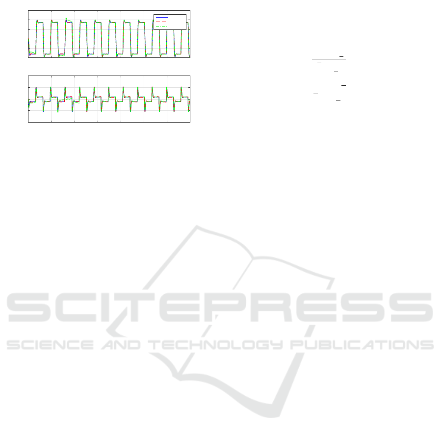
0 1000 2000 3000 4000 5000 6000 7000

-40

-20

State Estimation

Real

LPV-UIO

LPV-LU

Time(Steps)

0 1000 2000 3000 4000 5000 6000 7000

-400

-200

200

400

Figure 6: Loss of effectiveness parameters.

By deﬁning the auxiliary state

x(t) :=



(t) b(t) γ

(t) γ

(t)



the augmented model (9) is derived where

A =





A 0 0

0 1 0

0 0 I

3×3





B =





1×1

3×1





E =





1×1

3×1





F =





2×1

3×1





{γ(t),x

(t)}

= (40)







(t) 0 1 0 0 0

(t) γ

(t) 1 0 0 0

0 0 1 x

(t) 0 0

0 0 1 0 x

(t) 0

0 0 1 0 0 x

(t) + x

(t)







D =





2×3

1×3

3×3





(41)

In order to exploit a polytopic Luenberger observer

for (9), an embedding polytopic representation of the

form (14) has been derived. To this end, the matrix

γ,x

can be embedded in P

:= Co{C

,...,C

} with

related vertices computed by evaluating matrix

γ,x

on the extremum points of Γ and x

. Then, a suit-

able polytopic representation (14) can be achieved by

ﬁrst deriving the LPV scheduling parameter ρ(p), that

in this example is composed by 32 components, each

one having the following structure

∏

i, j

(1 − p

)(1 − p

)

∏

i, j

(42)

where the measurable parameters p

and p

obtained

by normalizing and centering the physical signals γ(t)

and x

(t)

(t) =

(t) − γ

− γ

, i = 1,.., 3

(t) =

(t) − x

− x

, j = 1,2 (43)

Finally, it is possible to get a polytopic embedding

approximation for

γ,x

as follows

∑

i=1

(p)C

(44)

A simulative comparison has been attempted between

the presented LPV-LU-SR scheme and the Sensor

Reconciliating approach of (Behzad et al., 2016), here

referred to as LPV-UIO-SR and endowed with a LPV

polytopic observer. In order to compute the observer’s

gain, the same embedding polytopic representation

used in (Behzad et al., 2016) has been here considered

for the matrix

, that consists in a polytope charac-

terized by 64 vertices.

In Figures 3-6 these schemes have been com-

pared. Although both observers achieve good perfor-

mance in getting an estimate of x

(1)

, as expected, the

LPV-LU-SR scheme exhibits a slight better behav-

ior with respect to LPV-UIO-SR, both in estimating

the state and the bias. This is mostly due to the fact

the observer exploits the knowledge on the input v(t)

supposed unknown in the case of the LPV-UIO-SR

scheme. Such an aspect translates in a better effec-

tiveness parameter (gain matrix) estimation (Figure 4)

and in a more accurate virtual output generation (Fig-

ure 6).

However, beyond the numerical results, it is worth

discussing some practical aspects of the considered

strategies. Unlikely the LPV-UIO-SR, the LPV-LU-

SR does not require any persistent excitation of the

state estimate that is needed to ensure parameter es-

timation convergence. Unfortunately, such an expe-

dient is not enough in general to guarantee conver-

gence on the state estimation. On the other hand, the

LPV-UIO-SR presents two advantages with respect

to LPV-LU-SR: it does not require neither the input

knowledge nor any pre-speciﬁed bounds on the state

7 CONCLUSIONS

In this paper, LPV Luenberger observers have been

proposed to solve fault-tolerant sensor reconciliation

A Fault-Tolerant Sensor Reconciliation Scheme based on Self-Tuning LPV Observers

117

design problems for linear discrete-time systems sub-

ject to possible faults on sensor gain and bias. The

role of the observer relies on the estimation of both

the state of the system and the current fault of the

physical sensors. The resulting design procedure is

quite simple and guarantees bounded errors on the es-

timation of both the plant state and fault parameters.

The scheme has been fully described, its properties

rigorously proved and, in the ﬁnal simulation exam-

ple, it has been shown to achieve good performance

in recovering useful data from the pool of redundant

sensors.

REFERENCES

Bara, G. I., Daafouz, J., Kratz, F., and Ragot, J. (2001).

“Parameter-dependent state observer design for afﬁne

LPV systems”. International Journal of Control,

74(16):1601–1611.

Behzad, H., Casavola, A., Tedesco, F., and Sadrnia, M. A.

(2016). “A fault-tolerant sensor reconciliation scheme

based on LPV Unknown Input Observers”. In IEEE

55th Conference on Decision and Control (CDC),

2016, Las Vegas, NV. IEEE.

Heemels, W. M. H., Daafouz, J., and Millerioux, G. (2010).

“Observer-based control of discrete-time LPV sys-

tems with uncertain parameters”. IEEE Trans. on Aut.

Contr., 55(9):2130–2135.

Lunze, J. and Richter, J. H. (2008). “Reconﬁgurable fault-

tolerant control: a tutorial introduction”. European

Journal of Control, 14(5):359–386.

Merrill, W. C., DeLaat, J. C., and Bruton, W. M. (1988).

“Advanced detection, isolation, and accommodation

of sensor failures-real-time evaluation”. Journal of

Guidance, Control, and Dynamics, 11(6):517–526.

Ponsart, J.-C., Theilliol, D., and Aubrun, C. (2010). “Vir-

tual sensors design for active fault tolerant control sys-

tem applied to a winding machine”. Control Engineer-

ing Practice, 18(9):1037–1044.

Samara, P. A., Fouskitakis, G. N., Sakellariou, J. S., and

Fassois, S. D. (2008). “A statistical method for the

detection of sensor abrupt faults in aircraft control sys-

tems”. IEEE Transactions on Control Systems Tech-

nology, 16(4):789–798.

Steffen, T. (2005). “Reconﬁguration using a virtual sen-

sor”. In Control Reconﬁguration of Dynamical Sys-

tems, pages 69–79. Springer.

Zhou, M., Shen, Y., and Wang, Q. (2013). “Robust UIO-

based fault estimation for sampled-data systems: An

LMI approach”. In IEEE International Conference

on Information and Automation (ICIA), 2013, pages

1308–1313, Yinchuan, China.

ICINCO 2018 - 15th International Conference on Informatics in Control, Automation and Robotics

118