
Quantitative Assessment of Robotic Swarm Coverage
Brendon G. Anderson
1
, Eva Loeser
2
, Marissa Gee
3
, Fei Ren
1
, Swagata Biswas
1
,
Olga Turanova
1
, Matt Haberland
1,∗
and Andrea L. Bertozzi
1
1
UCLA, Dept. of Mathematics, Los Angeles, CA 90095, U.S.A.
2
Brown University, Mathematics Department, Providence, RI 02912, U.S.A.
3
Harvey Mudd College, Dept. of Mathematics, Claremont, CA 91711, U.S.A.
Keywords:
Swarm Robotics, Multi-agent Systems, Coverage, Optimization, Central Limit Theorem.
Abstract:
This paper studies a generally applicable, sensitive, and intuitive error metric for the assessment of robotic
swarm density controller performance. Inspired by vortex blob numerical methods, it overcomes the shortco-
mings of a common strategy based on discretization, and unifies other continuous notions of coverage. We
present two benchmarks against which to compare the error metric value of a given swarm configuration: non-
trivial bounds on the error metric, and the probability density function of the error metric when robot positions
are sampled at random from the target swarm distribution. We give rigorous results that this probability density
function of the error metric obeys a central limit theorem, allowing for more efficient numerical approxima-
tion. For both of these benchmarks, we present supporting theory, computation methodology, examples, and
MATLAB implementation code.
1 INTRODUCTION
Much of the research in swarm robotics has focused
on determining control laws that elicit a desired group
behavior from a swarm (Brambilla et al., 2013), while
less attention has been placed on methods for quanti-
fying and evaluating the performance of these con-
trollers. Both (Brambilla et al., 2013) and (Cao et al.,
1997) point out the lack of developed performance
metrics for assessing and comparing swarm behavior,
and (Brambilla et al., 2013) notes that when perfor-
mance metrics are developed, they are often too spe-
cific to the task being studied to be useful in compa-
ring performance across controllers. This paper deve-
lops an error metric that evaluates one common desi-
red swarm behavior: distributing the swarm according
to a prescribed spatial density.
In many applications of swarm robotics, the
swarm must spread across a domain according to a
target distribution in order to achieve its goal. Some
examples are in surveillance and area coverage (Bru-
emmer et al., 2002; Hamann and W
¨
orn, 2006; Ho-
ward et al., 2002; Schwager et al., 2006), achie-
ving a heterogeneous target distribution (Elamvazhu-
thi et al., 2016; Berman et al., 2011; Demir et al.,
2015; Shen et al., 2004; Elamvazhuthi and Berman,
2015), and aggregation and pattern formation (Soy-
∗
Corresponding author: haberland@ucla.edu
sal and S¸ahin, 2006; Spears et al., 2004; Reif and
Wang, 1999; Sugihara and Suzuki, 1996). Despite
the importance of assessing performance, some stu-
dies such as (Shen et al., 2004) and (Sugihara and Su-
zuki, 1996) rely only on qualitative methods such as
visual comparison. Others present performance me-
trics that are too specific to be used outside of the
specific application, such as measuring cluster size in
(Soysal and S¸ahin, 2006), distance to a pre-computed
target location in (Schwager et al., 2006), and area
coverage by tracking the path of each agent in (Bru-
emmer et al., 2002). In (Reif and Wang, 1999) an L
2
norm of the difference between the target and achie-
ved swarm densities is considered, but the notion of
achieved swarm density is particular to the controllers
under study.
We develop and analyze an error metric that quan-
tifies how well a swarm achieves a prescribed spatial
distribution. Our method is independent of the con-
troller used to generate the swarm distribution, and
thus has the potential to be used in a diverse range of
robotics applications. In (Li et al., 2017) and (Zhang
et al., 2018), error metrics similar to the one presented
here are used, but their properties are not discussed in
sufficient detail for them to be widely adopted. In par-
ticular, although the error metric that we study always
takes values somewhere between 0 and 2, these values
are, in general, not achievable for an arbitrary desired
distribution and a fixed number of robots. How then,
Anderson, B., Loeser, E., Gee, M., Ren, F., Biswas, S., Turanova, O., Haberland, M. and Bertozzi, A.
Quantitative Assessment of Robotic Swarm Coverage.
DOI: 10.5220/0006844600910101
In Proceedings of the 15th International Conference on Informatics in Control, Automation and Robotics (ICINCO 2018) - Volume 2, pages 91-101
ISBN: 978-989-758-321-6
Copyright © 2018 by SCITEPRESS – Science and Technology Publications, Lda. All rights reserved
91

in general, is one to judge whether the value of the
error metric, and thus the robot distribution, achieved
by a given swarm control law is “good” or not? We
address this by studying two benchmarks,
1. the global extrema of the error metric, and
2. the probability density function (PDF) of the error
metric when robot positions are sampled from the
target distribution,
which were first proposed in (Li et al., 2017). Using
tools from nonlinear programming for (1) and ri-
gorous probability results for (2), we put each of these
benchmarks on a firm foundation. In addition, we
provide MATLAB code for performing all calculati-
ons at https://git.io/v5ytf. Thus, by using the methods
developed here, one can assess the performance of a
given controller for any target distribution by compa-
ring the error metric value of robot configurations pro-
duced by the controller against benchmarks (1) and
(2).
Our paper is organized as follows. Our main defi-
nition, its basic properties, and a comparison to com-
mon discretization methods is presented in Section 2.
Then, Section 3 and Section 4 are devoted to studying
(1) and (2), respectively. We suggest future work and
conclude in Section 5.
2 QUANTIFYING COVERAGE
One difficulty in quantifying swarm coverage is that
the target density within the domain is often pres-
cribed as a continuous (or piecewise continuous)
function, yet the swarm is actually composed of a fi-
nite number of robots at discrete locations. A com-
mon approach for comparing the actual positions of
robots to the target density function begins by discre-
tizing the domain (e.g. (Berman et al., 2011; Demir
et al., 2015)). We demonstrate the pitfalls of this in
Subsection 2.5. Another possible route (the one we
take here) is to use the robot positions to construct
a continuous function that represents coverage (e.g.
(Hussein and Stipanovic, 2007; Zhong and Cassan-
dras, 2011; Ayvali et al., 2017)). It is also possible to
use a combination of the two methods, as in (Cortes
et al., 2004).
The method we present and analyze is inspired by
vortex blob numerical methods for the Euler equa-
tion and the aggregation equation (see (Craig and Ber-
tozzi, 2016) and the references therein). A similar
strategy was used in (Li et al., 2017) and (Zhang et al.,
2018) to measure the effectiveness of a certain robo-
tic control law, but to our knowledge, our work is the
first study of any such method in a form sufficiently
general for common use.
2.1 Definition
We are given a bounded region
1
Ω ∈ R
d
, a desired ro-
bot distribution ρ : Ω → (0, ∞) satisfying
R
Ω
ρ(z)dz =
1, and N robot positions x
1
,...,x
N
∈ Ω. To compare
the discrete points x
1
,...x
N
to the function ρ, we place
a “blob” of some shape and size at each point x
i
. The
shape and size parameters have two physical interpre-
tations as:
• the area in which an individual robot performs its
task, or
• inherent uncertainty in the robot’s position.
Either of these interpretations (or a combination of the
two) can be invoked to make a meaningful choice of
these parameters.
The blob or robot blob function can be any
function K(z) : R
d
→ R that is non-negative on Ω and
satisfies
R
R
d
K(z)dz = 1. While not required, it is of-
ten natural to use a K that is radially symmetric and
decreasing along radial directions. In this case, we
need one more parameter, a positive number δ, that
controls how far the effective area (or inherent positi-
onal uncertainty) of the robot extends. We then define
K
δ
as,
K
δ
(z) =
1
δ
d
K
z
δ
. (1)
We point out that we still have
R
R
d
K
δ
(z)dz = 1. One
choice of K
δ
would be a scaled indicator function, for
instance, a function of constant value within a disc
of radius δ and 0 elsewhere. This is an appropriate
choice when a robot is considered to either perform
its task at a point or not, and where there is no notion
of the degree of its effectiveness. For the remainder
of this paper, however, we usually take K to be the
Gaussian
G(z) =
1
2π
exp
−
|z|
2
2
,
which is useful when the robot is most effective at
its task locally and to a lesser degree some distance
away. To define the swarm blob function ρ
δ
N
, we place
a blob G
δ
at each robot position x
i
, sum over i and
renormalize, yielding,
ρ
δ
N
(z;x
1
,...,x
N
) =
∑
N
i=1
G
δ
(z − x
i
)
∑
N
i=1
R
Ω
G
δ
(z − x
i
)dz
. (2)
1
We present our definitions for any number of dimensi-
ons d ≥ 1 to demonstrate their generality. However, in the
latter sections of the paper, we restrict ourselves to d = 2, a
common setting in ground-based applications.
ICINCO 2018 - 15th International Conference on Informatics in Control, Automation and Robotics
92

For brevity, we usually write ρ
δ
N
(z) to mean
ρ
δ
N
(z;x
1
,...,x
N
). This swarm blob function gives a
continuous representation of how the discrete robots
are distributed. Note that each integral in the denomi-
nator of (2) approaches 1 if δ is small or all robots are
far from the boundary, so that we have,
ρ
δ
N
(z) ≈
1
N
N
∑
i=1
G
δ
(z − x
i
). (3)
We now define our notion of error, which we refer
to as the error metric:
e
δ
N
(x
1
,...,x
N
) =
Z
Ω
ρ
δ
N
(z) − ρ(z)
dz. (4)
We often write this as e
δ
N
for brevity.
2.2 Remarks and Basic Properties
Our error is defined as the L
1
norm between the
swarm blob function and the desired robot distribu-
tion ρ. One could use another L
p
norm; however,
p = 1 is a standard choice in applications that involve
particle transportation and coverage such as (Zhang
et al., 2018). Moreover, the L
1
norm has a key pro-
perty: for any two integrable functions f and g,
Z
Ω
|
f − g
|
dz = 2 sup
B⊂Ω
Z
B
f dz −
Z
B
gdz
.
The other L
p
norms do not enjoy this property (De-
vroye and Gy
˝
orfi, 1985, Chapter 1). Consequently, by
measuring L
1
norm on Ω, we are also bounding the er-
ror we make on any particular subset, and, moreover,
knowing the error on “many” subsets gives an esti-
mate of the total error. This means that by using the
L
1
norm we capture the idea that discretizing the dom-
ain provides a measure of error, but avoid the pitfalls
of discretization methods described in Subsection 2.5.
Studies in optimal control of swarms often use the
L
2
norm due to the favorable inner product structure
(Zhang et al., 2018). We point out that the L
1
norm
is bounded from above by the L
2
norm due to the
Cauchy-Schwarz inequality and the fact that Ω is a
bounded region. Thus, if an optimal control strategy
controls the L
2
norm, then it will also control the error
metric we present here.
Last, we note:
Proposition 2.1. For any Ω, ρ, δ, N, and (x
1
,...,x
N
),
0 ≤ e
δ
N
≤ 2.
Proof. This follows directly from the basic property
Z
| f | dz−
Z
|g|dz ≤
Z
| f −g|dz ≤
Z
| f | dz+
Z
|g|dz
and our normalization.
The theoretical minimum of e
δ
N
can only be appro-
ached for a general target distribution when δ is small
and N is large, or in the trivial special case when the
target distribution is exactly the sum of N Gaussians
of the given δ, motivating the need to develop bench-
marks (1) and (2).
2.3 Variants of the Error Metric
The notion of error defined by (4) is suitable for tasks
that require good instantaneous coverage. For tasks
that involve tracking average coverage over some pe-
riod of time (and in which the robot positions are
functions of time t), an alternative “cumulative” ver-
sion of the error metric is
Z
Ω
1
M
M
∑
j=1
ρ
δ
N
(z,t
j
) − ρ
Ω
(z)
dz (5)
for time points j = 1, . . . , M. This is a practical,
discrete-time version of the metric used in (Zhang
et al., 2018), which uses a time integral rather than
a sum, as in practice, position measurements can only
be made at discrete times. While this cumulative error
metric is, in general, distinct from the instantaneous
version of (4), note that the extrema and PDF of this
cumulative version can be calculated as the extrema
and PDF of the instantaneous error metric with MN
robots. Therefore, in subsequent sections we restrict
our attention to the extrema and PDF of the instanta-
neous formulation without loss of generality.
In addition, (Zhang et al., 2018) considers a one-
sided notion of error, in which a scarcity of robots is
penalized but an excess is not, that is,
ˆe
δ
N
=
Z
Ω
−
ρ
δ
N
(z) − ρ(z)
dz,
where Ω
−
:= {z|ρ
δ
N
(z) ≤ ρ(z)}. Remarkably, ˆe
δ
N
and
e
δ
N
are related by:
Proposition 2.2. e
δ
N
= 2 ˆe
δ
N
.
Proof. Let Ω
+
= Ω \ Ω
−
. Since Ω = Ω
−
∪ Ω
+
, we
have,
Z
Ω
−
ρ
δ
N
dz +
Z
Ω
+
ρ
δ
N
dz =
Z
Ω
ρ
δ
N
dz = 1 =
=
Z
Ω
ρdz =
Z
Ω
−
ρdz +
Z
Ω
+
ρdz.
Rearranging and taking absolute values we find
Z
Ω
−
ρ
δ
N
− ρ
dz =
Z
Ω
+
ρ
δ
N
− ρ
dz,
as each integrand is of the same sign everywhere
within the limits of integration. We notice that the
left-hand side and therefore the right-hand side of the
previous line equal ˆe
δ
N
. On the other hand, their sum
equals e
δ
N
. Thus our claim holds.
Quantitative Assessment of Robotic Swarm Coverage
93

The definition of ˆe
δ
N
is particularly useful in con-
junction with the choice of K
δ
as a scaled indicator
function, as ˆe
δ
N
becomes a direct measure of the defi-
ciency in coverage of a robotic swarm. For instance,
given a swarm of surveillance robots, each with obser-
vational radius δ, ˆe
δ
N
is the percentage of the domain
not observed by the swarm.
2
Proposition 2.2 implies
that
1
2
e
δ
N
also enjoys this interpretation.
2.4 Calculating e
δ
N
In practice, the integral in (4) can rarely be carried
out analytically, primarily because the integral needs
to be separated into regions for which the quantity
ρ
δ
N
(z)−ρ(z) is positive and regions for which it is ne-
gative, the boundaries between which are usually dif-
ficult to express in closed form. We find that a simple
generalization of the familiar rectangle rule converges
linearly in dimensions d ≤ 3 and expect Monte Carlo
and Quasi-Monte Carlo methods to produce a reaso-
nable estimate in higher dimensions
3
. More advanced
quadrature rules can be used in low dimensions, but
may suffer in accuracy due to nonsmoothness in the
target distribution and/or stemming from the absolute
value taken within the integral.
2.5 The Pitfalls of Discretization
We conclude this section by analyzing a measure of
error that involves discretizing the domain. In parti-
cular, we show in Propositions 2.3 and 2.4 that the va-
lues produced by this method are strongly dependent
on a choice of discretization. In particular, this er-
ror approaches its theoretical minimum when the dis-
cretization is too coarse and its theoretical maximum
when the discretization is too fine, regardless of robot
positions.
Discretizing the domain means dividing Ω into
M disjoint regions Ω
i
⊂ Ω such that
S
M
i=1
Ω
i
= Ω.
Within each region, the desired proportion of robots
is the integral of the target density function within the
region
R
Ω
i
ρ(z)dz. Using N
i
to denote the observed
number of robots in Ω
i
, we can define an error metric
as
µ =
M
∑
i=1
Z
Ω
i
ρ(z)dz −
N
i
N
. (6)
2
The notion of “coverage” in (Bruemmer et al., 2002)
might be interpreted as ˆe
δ
N
with δ as the width of the robot.
There, only the time to complete coverage ( ˆe
δ
N
= 0) was
considered.
3
We look forward to a physical swarm of robots being
deployed – and these results employed – in four dimensi-
ons!
It is easy to check that 0 ≤ µ ≤ 2 always holds. One
advantage of this approach is that µ is very easy to
compute, but there are two major drawbacks.
2.5.1 Choice of Domain Discretization
The choice for domain discretization is not unique,
and this choice can dramatically affect the value of µ,
as demonstrated by the following two propositions.
Proposition 2.3. If M = 1 then µ = 0.
Proof. When M = 1, (6) becomes
µ =
Z
Ω
ρ(z)dz − 1
= 0.
The situation of perfectly fine discretization is in
complete contrast.
Proposition 2.4. Suppose the robot positions are dis-
tinct
4
and the regions Ω
i
are sufficiently small such
that, for each i, Ω
i
contains at most one robot and
R
Ω
i
ρ(z)dz ≤ 1/N holds. Then µ → 2 as |Ω
i
| → 0.
Proof. Let us relabel the Ω
i
so that for i = 1, ..., M −N
there is no robot in Ω
i
, and thus each of the Ω
i
for
i = M − N + 1, ..., M contains exactly one robot. In
this case, the expression for error µ becomes,
µ =
M−N
∑
i=1
Z
Ω
i
ρdz +
M
∑
i=M−N+1
Z
Ω
i
ρdz −
1
N
. (7)
Since
R
Ω
i
ρdz ≤ 1/N holds, then with the identity
M−N
∑
i=1
Z
Ω
i
ρdz = 1 −
M
∑
i=M−N+1
Z
Ω
i
ρdz,
we can rewrite (7) as,
µ = 1−
M
∑
i=M−N+1
Z
Ω
i
ρdz +
M
∑
i=M−N+1
1
N
−
Z
Ω
i
ρdz
= 2 − 2
M
∑
i=M−N+1
Z
Ω
i
ρdz.
Thus µ → 2 as M → ∞ and |Ω
i
| → 0.
Note that the shape of each region is also a choice
that will affect the calculated value. While our appro-
ach also requires the choice of some size and shape
(namely, δ and K), these parameters have much more
immediate physical interpretation, making appropri-
ate choices easier to make.
4
This is reasonable in practice as two physical robots
cannot occupy the same point in space. In addition, the
proof can be modified to produce the same result even if
the robot positions coincide.
ICINCO 2018 - 15th International Conference on Informatics in Control, Automation and Robotics
94

2.5.2 Error Metric Discretization and
Desensitization
Perhaps more importantly, by discretizing the dom-
ain, we also discretize the range of values that the the
error metric can assume. While this may not be inhe-
rently problematic, we have simultaneously desensi-
tized the error metric to changes in robot distribution
within each region. That is, as long as the number of
robots N
i
within each region Ω
i
does not change, the
distribution of robots within any and all Ω
i
may be
changed arbitrarily without affecting the value of µ.
On the other hand, the error metric e
δ
N
is continuously
sensitive to differences in distribution.
3 ERROR METRIC EXTREMA
In the rest of the paper, we provide tools for determi-
ning whether or not the values of e
δ
N
produced by a
controller in a given situation are “good”. As mentio-
ned in Section 2.2, it is simply not possible to achieve
e
δ
N
= 0 for every combination of target distribution
ρ, number of robots N, and blob size δ . Therefore,
we would like to compare the achieved value of e
δ
N
against its realizable extrema given ρ, N, and δ. But
e
δ
N
is a highly nonlinear function of the robot positions
(x
1
,...,x
N
), and trying to find its extrema analytically
has been intractable. Thus, we approach this problem
by using nonlinear programming.
3.1 Extrema Bounds via Nonlinear
Programming
Let x = (x
1
,...,x
N
) represent a vector of N robot coor-
dinates. The optimization problem is
minimize e
δ
N
(x
1
,...,x
N
), (8)
subject to x
i
∈ Ω for i ∈ {1, 2, . . . ,N}.
Note that the same problem structure can be used
to find the maximum of the error metric by minimi-
zing −e
δ
N
. Given ρ, N, and δ, we solve these pro-
blems using a standard nonlinear programming sol-
ver, MATLAB’s fmincon.
A limitation of all general nonlinear program-
ming algorithms is that successful termination produ-
ces only a local minimum, which is not guaranteed
to be the global minimum. There is no obvious re-
formulation of this problem for which a global solu-
tion is guaranteed, so the best we can do is to use a
local minimum produced by nonlinear programming
as an upper bound for the minimum of the error me-
tric. Heuristics, such as multi-start (running the opti-
mization many times from several initial guesses and
taking the minimum of the local minima) can be used
to make this bound tighter. This bound, which we call
e
−
, and the equivalent bound on the maximum, e
+
,
serve as benchmarks against which we can compare
an achieved value of the error metric. This is reasona-
ble, because if a configuration of robots with a lower
value of the error metric exists but eludes numerical
optimization, it is probably not a fair standard against
which to compare the performance of a general con-
troller.
3.2 Relative Error
The performance of a robot distribution controller can
be quantitatively assessed by calculating the error va-
lue e
observed
of a robot configuration it produces, and
comparing this value against the extrema bounds e
−
and e
+
. If the robot positions x
1
,...,x
N
produced by
a given controller are constant, then e
observed
can sim-
ply be taken as e
δ
N
(x
1
,...,x
N
). In general, however,
the positions x
1
,...,x
N
may change over time. In this
case, we suggest using the third-quartile value obser-
ved after the system reaches steady state, which we
denote e
Q3
.
Consider the relative error
e
rel
=
e
observed
− e
−
e
+
− e
−
.
We suggest that if e
rel
is less than 10%, the perfor-
mance of the controller is quite close to the best pos-
sible, whereas if this ratio is 30% or higher, the per-
formance of the controller is rather poor.
3.3 Example
We apply this method to assess the performance of the
controller in (Li et al., 2017), which guides a swarm
of N = 200 robots with δ = 2in (the physical radius
of the robots) to achieve a “ring distribution”
5
.
Under this stochastic control law, the behavior
of the error metric over time appears to be a noisy
decaying exponential. Therefore, we fit to the data
shown in Figure 7 of (Li et al., 2017) a function of the
form f (t) = α + β exp(−
t
τ
) by finding error asymp-
tote α, error range β, and time constant τ that mi-
nimize the sum of squares of residuals between f (t)
and the data. By convention, the steady state settling
5
The ring distribution ρ
ring
is defined on the Cartesian
plane with coordinates z = (z
1
,z
2
) as follows. Let inner ra-
dius r
1
= 11.4in, outer radius r
2
= 20.6in, width w = 48in,
height h = 70in, and ρ
0
= 2.79 × 10
−5
. Let domain Ω =
{z : z
1
∈ [0, w],z
2
∈ [0, h]} and region Γ = {z : r
2
1
< (z
1
−
w
2
)
2
+ (z
2
−
h
2
)
2
< r
2
2
}. Then ρ
ring
(z) = 36ρ
0
if z ∈ Ω ∩ Γ,
ρ
0
if z ∈ Ω \ Γ.
Quantitative Assessment of Robotic Swarm Coverage
95
time is taken to be t
s
= 4τ, which can be interpreted
as the time at which the error has settled to within 2%
of its asymptotic value (Barbosa et al., 2004). The
third quartile value of the error metric for t > t
s
is
e
Q3
= 0.5157.
To determine an upper bound on the global mini-
mum of the error metric, we computed 50 local mi-
nima of the error metric starting with random initial
guesses, then took the lowest of these to be e
−
=
0.28205. An equivalent procedure bounds the global
maximum as e
+
= 1.9867, produced when all robot
positions coincide near a corner of the domain. The
corresponding swarm blob functions are depicted in
Figures 1 and 2. Note that the minimum of the error
metric is significantly higher than zero for this finite
number of robots of nonzero radius, emphasizing the
importance of performing this benchmark calculation
rather than using zero as a reference.
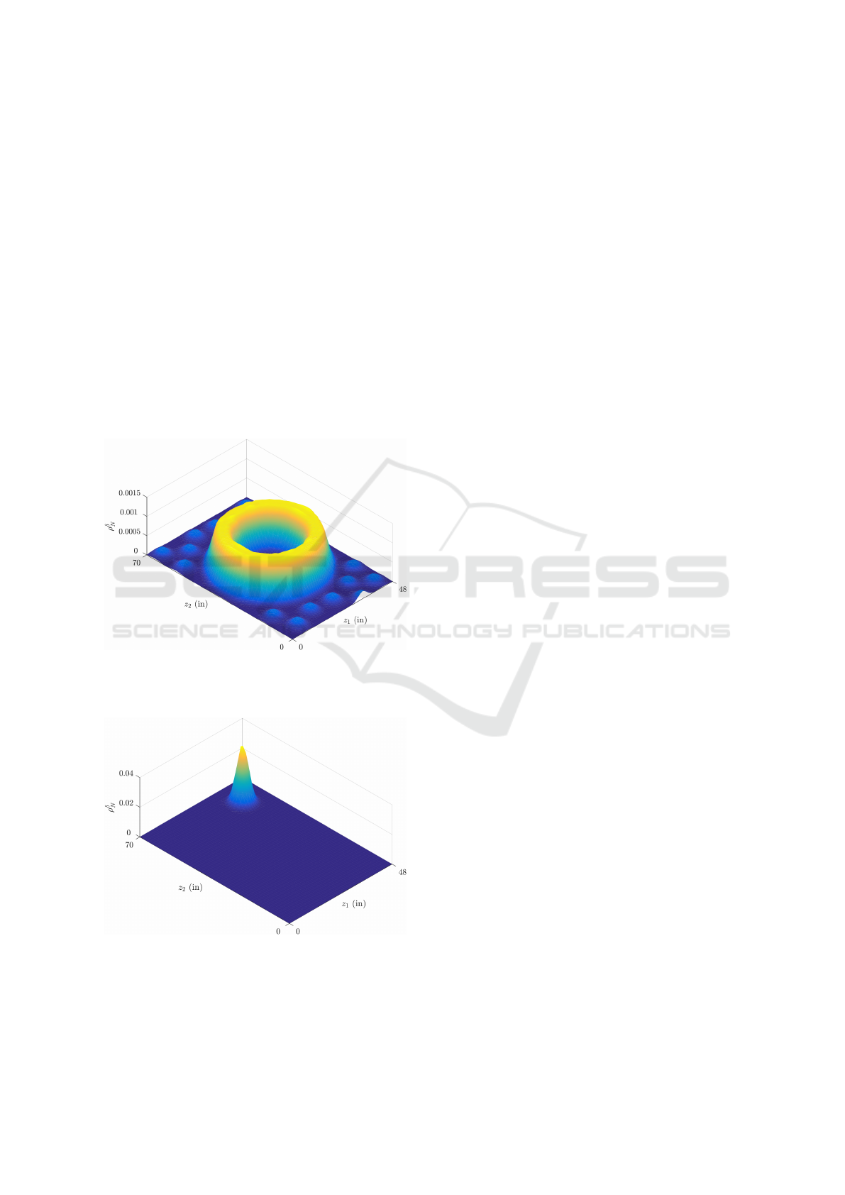
Figure 1: Swarm blob function ρ
δ=2in
N=200
corresponding with
the robot distribution that yields a minimum value of the
error metric for the ring distribution, 0.28205.
Figure 2: Swarm blob function ρ
δ=2in
N=200
corresponding with
the robot distribution that yields a maximum value of the
error metric for the ring distribution, 1.9867. This occurs
when all robots coincide outside the ring.
Using these values for e
Q3
, e
−
, and e
+
, we calcu-
late e
rel
according to Equation 3.2 as 13.71%.
While the sentiment of the e
rel
benchmark is found
in (Li et al., 2017), we have made three important im-
provements to the calculation to make it suitable for
general use. First, in (Li et al., 2017) values analo-
gous to e
−
and e
+
were found by “manual placement”
of robots, whereas we have used nonlinear program-
ming so that the calculation is objective and repeata-
ble. Second, (Li et al., 2017) refers to steady state but
does not suggest a definition. Adopting the 2% sett-
ling time convention not only allows for an unambi-
guous calculation of e
Q3
and other steady-state error
metric statistics, but provides a metric for assessing
the speed with which the control law effects the de-
sired distribution. Finally, (Li et al., 2017) uses the
minimum observed value of the error metric in the
calculation, but we suggest that the third quartile va-
lue better represents the distribution of error metric
values achieved by a controller, and thus is more re-
presentative of the controller’s overall performance.
These changes account for the difference between
our calculated value of e
rel
= 13.71% and the report
in (Li et al., 2017) that the error is “7.2% of the range
between the minimum error value . . . and maximum
error value”. Our substantially higher value of e
rel
indicates that the performance of this controller is
not very close the best possible. We emphasize this
to motivate the need for our second benchmark in
Section 4, which is more appropriate for a stochastic
controller like the one presented in (Li et al., 2017).
3.4 Error Metric for Optimal Swarm
Design
So far we have taken N and δ to be fixed; we have
assumed that the robotic agents and size of the swarm
have already been chosen. We briefly consider the use
of the error metric as an objective function for the de-
sign of a swarm. Simply adding δ > 0 as a decision
variable to (8) and solving at several fixed values of
N provides insight into how many robots of what ef-
fective working radius are needed to achieve a given
level of coverage for a particular target distribution.
Visualizations of such calculations are provided in Fi-
gure 3 and the supplemental video.
Note that ‘breakthroughs’, or relatively rapid de-
creases in the error metric, can occur once a critical
number of robots are available; these correspond with
a qualitative change in the distribution of robots. For
example, at N = 22 the robots are arranged in a sin-
gle ring; beginning with N = 25 we see the robots
begin to be arranged in two separate concentric rings
of different radii and the error metric begins to drop
ICINCO 2018 - 15th International Conference on Informatics in Control, Automation and Robotics
96
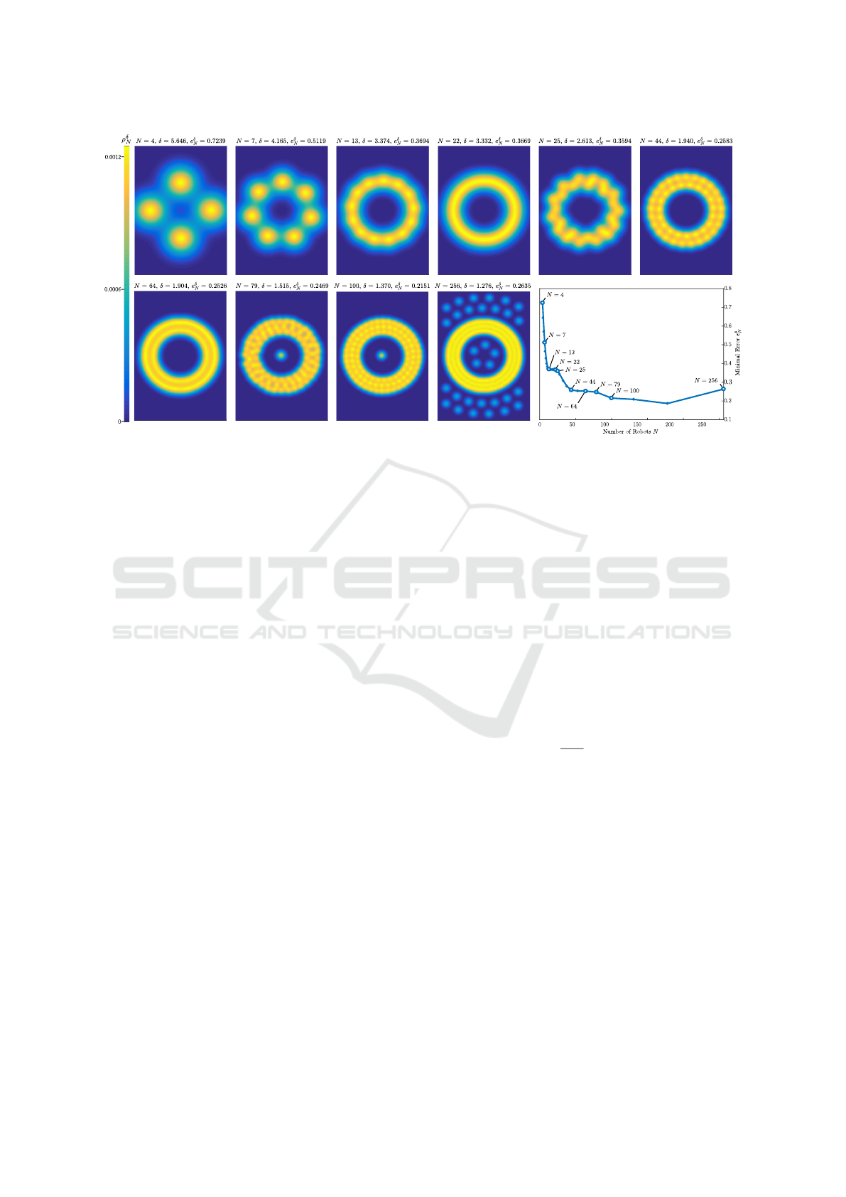
Figure 3: Swarm blob functions ρ
δ
N
corresponding with the robot distributions and values of δ that yield the minimum value
of the error metric for the ring distribution target. Inset graph shows the relationship between N and the minimum value of the
error metric observed from repeated numerical optimization. Due to long execution time of optimization at N = 256, fewer
local minima were calculated; this likely explain the rise in the minimal error metric value. This highlights the need in future
work to find a more efficient formulation of this optimization problem or to use a more effective solver.
sharply. On a related note, there are also “lulls” in
which increasing the number of robots has little ef-
fect on the minimum value of the error metric, such
as between N = 44 and N = 79. Studies like these
can help a swarm designer determine the best number
of robots N and effective radius of each δ to achieve
the required coverage.
4 ERROR METRIC
PROBABILITY DENSITY
FUNCTION
In the previous section we have described how to find
bounds on the minimum and maximum values for er-
ror. A question that remains is, how “easy” or “dif-
ficult” is it to achieve such values? Answering this
question is important in order to use the error metric
to assess the effectiveness of an underlying control
law. Indeed, a given control law — especially a sto-
chastic control law — may tend to produce robot po-
sitions with error well above the minimum, and it is
necessary to assess these values as well.
According to the setup of our problem, the goal of
any such control law is for the robots to achieve the
desired distribution ρ. Thus, whatever the particular
control law is, it is natural to compare its outcome
to simply picking the robot positions at random from
the target distribution ρ. In this section we consider
the robot positions as being sampled directly from the
desired distribution and study the statistical properties
of the error metric in this situation, both analytically
and numerically, and suggest how they may be used as
a benchmark with which to evaluate the performance
of a swarm distribution controller.
We take the robots’ positions X
1
, . . . , X
N
, to be
independent, identically distributed bivariate random
vectors in Ω ⊂ R
2
with probability density function
ρ. We place a blob of shape K at each of the X
i
(pre-
viously we took K to be the Gaussian G), so that the
swarm blob function is,
ρ
δ
N
(z) =
1
Nδ
2
N
∑
i=1
K
δ
(z − X
i
), (9)
where K
δ
is defined by (1). We point out that the
right-hand side of (9) is exactly that of (3) upon ta-
king K to be the Gaussian G and the robot locations
x
i
to be the randomly selected X
i
. The error e
δ
N
is now
a random variable, the value of which depends on the
particular realization of the robot positions X
1
, . . . ,
X
N
, but which has a well-defined probability density
function (PDF) and cumulative distribution function
(CDF). We denote the PDF and CDF by f
e
δ
N
and F
e
δ
N
,
respectively. The performance of a stochastic robot
distribution controller can be quantitatively assessed
by calculating the error values e
δ
N
(x
1
,...,x
N
) it produ-
ces in steady state and comparing their distribution to
f
e
δ
N
.
In Subsection 4.1 we present rigorous results that
Quantitative Assessment of Robotic Swarm Coverage
97

show that the error metric has an approximately nor-
mal distribution in this case. As a corollary we obtain
that the limit of this error is zero as N approaches in-
finity and δ approaches 0. Subsections 4.2 and 4.3
include a numerical demonstration of these results. In
addition, in 4.3, we present an example calculation.
The theoretical results presented in the next sub-
section not only support our numerical findings, they
also allow for faster computation. Indeed, if one did
not already know that the error when robots are sam-
pled randomly from ρ has a normal distribution for
large N, tremendous computation may be needed to
get an accurate estimate of this probability density
function. On the other hand, since the results we pre-
sent prove that the error metric has a normal distribu-
tion for large N, we need only fit a Gaussian function
to the results of relatively little computation.
4.1 Theoretical Central Limit Theorem
The expression (9) is the so-called kernel density esti-
mator of ρ. This arises in statistics, where ρ is thought
of as unknown, and ρ
δ
N
is considered as an approxima-
tion to ρ. It turns out that, under appropriate hypothe-
ses, the L
1
error between ρ and ρ
δ
N
has a normal dis-
tribution with mean and variance that approach zero
as N approaches infinity. In other words, a central li-
mit theorem holds for the error. For such a result to
hold, δ and N have to be compatible. Thus, for the
remainder of this subsection δ will depend on N, and
we display this as δ(N). We have,
Theorem 4.1. Suppose ρ is continuously twice diffe-
rentiable, K is zero outside of some bounded region
and radially symmetric. Then, for δ(N) satisfying
δ(N) = O(N
−1/6
) and lim
N→∞
δ(N)N
1/4
= ∞, (10)
we have
e
δ(N)
N
≈ N
e(N)
N
1/2
,
σ(N)
2
δ(N)
2
N
,
where σ
2
(N) and e(N) are deterministic quantities
that are bounded uniformly in N.
6
Proof. This follows from Horv
´
ath (Horv
´
ath, 1991,
Theorem, page 1935). For the convenience of the re-
ader, we record that the quantities N, δ, ρ, ρ
δ
N
, e
δ
N
that
we use here correspond to n, h, f , f
n
, I
n
in (Horv
´
ath,
1991). We do not present the exact expressions for
6
Here N (µ,σ
2
) denotes the normal random variable of
mean µ and variance σ
2
, and we use the notation ≈ to mean
that the difference of the quantity on the left-hand side and
on the right-hand side converges to zero in the sense of dis-
tributions as N → ∞.
σ(N) and e(N); they are written in (Horv
´
ath, 1991,
page 1934). The uniform boundedness of σ is ex-
actly line (1.2) of (Horv
´
ath, 1991); the boundedness
for e(N) is not written explicitly in (Horv
´
ath, 1991)
so we briefly explain how to derive it. In the expres-
sion for e(N) in (Horv
´
ath, 1991), m
N
is the only term
that depends on N. A standard argument that uses the
Taylor expansion of ρ and the symmetry of the kernel
K (see, for example, Section 2.4 of the lecture notes
(Hansen, 2009)) yields that m
N
is uniformly bounded
in N.
From this it is easy to deduce:
Corollary 4.2. Under the hypotheses of Theorem 4.1,
the error e
δ(N)
N
converges in distribution to zero as
N → ∞.
Remark 4.3. There are a few ways in which practical
situations may not align perfectly with the assumpti-
ons of (Horv
´
ath, 1991). However, we posit that in all
of these cases, the difference between these situati-
ons and that studied in (Horv
´
ath, 1991) is numerically
insignificant. We now briefly summarize these three
discrepancies and indicate how to resolve them.
First, we defined our density ρ
δ
N
by (2), but in this
section we use a version with denominator N. Howe-
ver, as explained above, the two expressions approach
each other for small δ, and this is the situation we are
interested in here. Second, a ρ that is piecewise conti-
nuous like the ring distribution is not twice differenti-
able. We point out that an arbitrary density ρ may be
approximated to arbitrary precision by a smoothed out
version, for example by convolution with a mollifier
(a standard reference is Brezis (Brezis, 2010, Section
4.4)). Third, in our computations we use the kernel
G, which is not compactly supported, for the sake of
simplicity. Similarly, this kernel can be approxima-
ted, with arbitrary accuracy, by a compactly supported
version. Making these changes to the kernel or target
density would not affect the conclusions of numerical
results.
4.2 Numerical Approximation of the
Error Metric PDF
In this subsection we describe how to numerically find
f
e
δ
N
and F
e
δ
N
. For sufficiently large N, one could sim-
ply use random sampling to estimate the mean and
standard deviation, then take these as the parameters
of the normal PDF (i.e. the error function and Gaus-
sian function, respectively). However, for moderate
N, we choose to begin by estimating the entire CDF
and confirming that it is approximately normal. We
first establish:
ICINCO 2018 - 15th International Conference on Informatics in Control, Automation and Robotics
98
Proposition 4.4. We have,
F
e
δ
N
(z) =
Z
Ω
N
1
{x|e
δ
N
(x)≤z}
N
∏
i=1
ρ(x
i
)dx. (11)
Proof. We recall a basic probability fact. Let Y be a
random vector with values in A ⊂ R
D
with probability
density function f , and let g be a real-valued function
on R
d
. The CDF for g(Y ), denoted F
g(Y )
, is given by,
F
g(Y )
(z) = P(g(Y ) ≤ z) =
Z
A
1
{y|g(y)≤z}
f (y)dy, (12)
where 1 denotes the indicator function.
In our situation, we take the random vector Y to
be X := (X
1
,...,X
N
). Since X takes values in Ω
N
:=
Ω×...×Ω, we take A to be Ω
N
(we point out that here
D = 2N). Since each X
i
has density ρ, the density of
X is the function
˜
ρ, defined by,
˜
ρ(x
1
,...,x
n
) =
N
∏
i=1
ρ(x
i
).
Thus, taking f and g in (12) to be
˜
ρ and e
δ
N
, respecti-
vely, yields (11).
Notice that since each of the x
i
is itself a 2-
dimensional vector (the X
i
are random points in the
plane and we are using the notation x = (x
1
,...,x
N
)),
the integral defining the cumulative distribution
function of the error metric is of dimension 2N. Fin-
ding analytical representations for the CDF is com-
binatorially complex and quickly becomes infeasible
for large swarms. Therefore, we approximate (11)
using Monte Carlo integration, which is well-suited
for high-dimensional integration (Sloan, 2010)
7
, and
fit a Gauss error function to the data. If the fitted curve
matches the data well, we differentiate to obtain the
PDF. We remark that we have used the notation of an
indicator function above in order to express the quan-
tity of interest in a way that is easily approximated
with Monte Carlo integration.
4.3 Example
We apply this method to assess the performance of
the controller in (Li et al., 2017), again for the “ring
distribution” scenario with N = 200 robots described
in Section 3.3.
7
Quasi-Monte Carlo techniques, which use a low-
discrepancy sequence rather than truly random evaluation
points, promise somewhat faster convergence but require
considerably greater effort to implement. The difficulty is
in generating a low-discrepancy sequence from the desired
distribution, which is possible using the Hlawka-M
¨
uck met-
hod, but computationally expensive (Hartinger and Kainho-
fer, 2006).
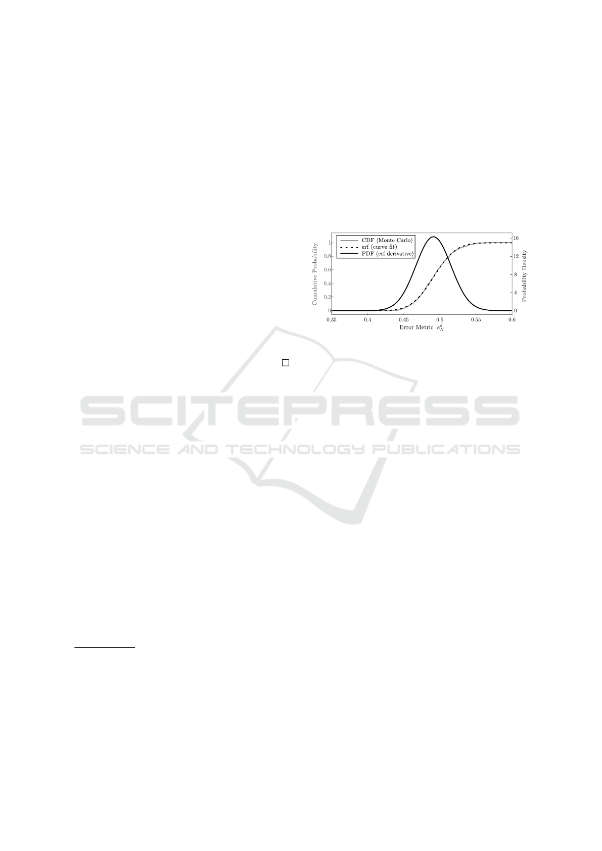
We approximate F
e
δ
N
using M = 1000 Monte Carlo
evaluation points; this is shown by a solid gray line
in Figure 4. The numerical approximation appears to
closely match a Gauss error function (erf(·), the inte-
gral of a Gaussian G) as theory predicts. Therefore an
analytical erf(·) curve, represented by the dashed line,
is fit to the data using MATLAB’s least squares curve
fitting routine lsqcurvefit. To obtain f
e
δ
N
, the ana-
lytical curve fit for F
e
δ
N
is differentiated, and the result
is also shown in Figure 4.
Figure 4: The CDF of the error metric when robot positi-
ons are sampled from ρ is approximated by Monte Carlo
integration, an erf curve fit matches closely, and the PDF is
taken as the derivative of the fitted erf.
With the error metric distribution now confirmed
to be approximately normal, the F- and T-tests (Moore
et al., 2009) are appropriate statistical procedures for
comparing the steady state error distribution to f
e
δ
N
.
From data presented as Figure 7 of (Li et al.,
2017), we calculate the distribution of steady state er-
ror metric values produced by the controller to have a
mean of 0.5026 with a standard deviation of 0.02586.
We take the null hypothesis to be that the distribution
of these error metric values is the same as f
e
δ
N
, which
has a sample mean of 0.4933 and a standard deviation
of 0.02484, as calculated from the M = 1000 samples.
A two-sample F-test fails to refute the null hypothesis,
with an F-statistic of 1.0831, indicating no significant
difference in the standard deviations. On the other
hand, a two-sample T-test rejects the null hypothesis
with a T-statistic of 8.5888, indicating that the steady
state error is not distributed with the same population
mean as f
e
δ
N
. However, the 95% confidence interval
for the true difference between population means is
computed to be (0.00717,0.01141), showing that the
mean steady state error achieved by this controller is
unlikely to exceed that of f
e
δ
N
by more than 2.31%.
Therefore, we find the performance of the controller
in (Li et al., 2017) to be acceptable given its stochas-
tic nature, as the error metric values it realizes are
only slightly different from those produced by sam-
pling robot positions from the target distribution.
As with e
rel
of Section 3, the sentiment of this ben-
Quantitative Assessment of Robotic Swarm Coverage
99

chmark is preceded by (Li et al., 2017). However, wit-
hout prior knowledge that f
e
δ
N
would be approxima-
tely Gaussian, the calculation took two orders of mag-
nitude more computation in that study
8
. Also, where
it is noted in (Li et al., 2017) that “the error values
[from simulation] mostly lie between . . . the 25th and
75th percentile error values when robot configurations
are randomly sampled from the target distribution”,
we have replaced visual inspection with the appropri-
ate statistical tests for comparing two approximately
normal distributions. These improvements make this
error metric PDF benchmark objective and efficient,
and thus suitable for common use.
5 FUTURE WORK AND
CONCLUSION
While the concepts presented herein are expected
to be sufficient for the comparison and evaluation
of swarm distribution controllers, the computational
techniques are certainly open to analysis and impro-
vement. For instance, is there a simpler, deterministic
method of approximating the error metric PDF f
e
δ
N
?
Is there a more appropriate formulation for determi-
ning the extrema of the error metric for a given si-
tuation, one that is guaranteed to produce a global
optimum? If not, which nonlinear programming al-
gorithm is most suitable for solving (8)? In practice,
what method of quadrature converges most efficiently
to approximate the error metric? As the size of practi-
cal robot swarms will likely grow faster than pro-
cessor speeds will increase, improved computational
techniques will be needed to keep benchmark compu-
tations practical.
Also, a very important question remains about the
nature of the error metric. The blob shape K
δ
has an
intuitive physical interpretation, and so a reasonable
choice is typically easy to make. The value of the
error metric for a particular situation is certainly af-
fected by the choice of blob shape K and radius δ, but
so are the values of the proposed benchmarks: the ex-
trema and the error PDF. Are qualitative conclusions
made by comparing the performance of the control-
ler to these benchmarks likely to be affected by the
choice of blob?
Open questions notwithstanding, the error metric
presented herein is sufficiently general to be used
in quantifying the the performance of one of the
most fundamental tasks of a robotic swarm controller:
8
According to the caption of Figure 2 of (Li et al., 2017),
the figure was generated as a histogram from 100,000
Monte Carlo samples.
achieving a prescribed density distribution. The error
metric is sensitive enough to compare the effective-
ness of given control laws for achieving a given target
distribution. The error metric parameters, blob shape
and radius, have intuitive physical interpretations so
that they can be chosen appropriately. Should a de-
signer wish to interpret the performance of a given
controller without comparing against results of anot-
her controller, we provide two benchmarks that can
be applied to any situation: extrema of the error me-
tric, and the probability density function of the error
metric when swarm configurations are sampled from
the target distribution. Using the provided code, these
methods can easily be used to quantitatively assess the
performance of new swarm controllers and thereby
improve the effectiveness of practical robot swarms.
ACKNOWLEDGEMENTS
The authors gratefully acknowledge the support
of NSF grant CMMI-1435709, NSF grant DMS-
1502253, the Dept. of Mathematics at UCLA, and
the Dept. of Mathematics at Harvey Mudd College.
The authors also thank Hao Li (UCLA) for his insig-
htful contributions regarding the connection between
this error metric and kernel density estimation.
REFERENCES
Ayvali, E., Salman, H., and Choset, H. (2017). Ergodic
coverage in constrained environments using stochas-
tic trajectory optimization. In Intelligent Robots and
Systems (IROS), 2017 IEEE/RSJ International Confe-
rence on. IEEE.
Barbosa, R. S., Machado, J. T., and Ferreira, I. M. (2004).
Tuning of PID controllers based on Bode’s ideal trans-
fer function. Nonlinear dynamics, 38(1):305–321.
Berman, S., Kumar, V., and Nagpal, R. (2011). Design
of control policies for spatially inhomogeneous robot
swarms with application to commercial pollination. In
Robotics and Automation (ICRA), 2011 IEEE Interna-
tional Conference on, pages 378–385. IEEE.
Brambilla, M., Ferrante, E., Birattari, M., and Dorigo, M.
(2013). Swarm robotics: a review from the swarm
engineering perspective. Swarm Intelligence, 7(1):1–
41.
Brezis, H. (2010). Functional analysis, Sobolev spaces and
partial differential equations. Springer Science & Bu-
siness Media.
Bruemmer, D. J., Dudenhoeffer, D. D., McKay, M. D., and
Anderson, M. O. (2002). A robotic swarm for spill fin-
ding and perimeter formation. Technical report, Idaho
National Engineering and Environmental Lab, Idaho
Falls.
ICINCO 2018 - 15th International Conference on Informatics in Control, Automation and Robotics
100

Cao, Y. U., Fukunaga, A. S., and Kahng, A. (1997). Coope-
rative mobile robotics: Antecedents and directions.
Autonomous robots, 4(1):7–27.
Cortes, J., Martinez, S., Karatas, T., and Bullo, F. (2004).
Coverage control for mobile sensing networks. IEEE
Transactions on Robotics and Automation.
Craig, K. and Bertozzi, A. (2016). A blob method for the
aggregation equation. Mathematics of computation,
85(300):1681–1717.
Demir, N., Eren, U., and Ac¸ıkmes¸e, B. (2015). Decen-
tralized probabilistic density control of autonomous
swarms with safety constraints. Autonomous Robots,
39(4):537–554.
Devroye, L. and Gy
˝
orfi, L. (1985). Nonparametric density
estimation: the L
1
view. Wiley.
Elamvazhuthi, K., Adams, C., and Berman, S. (2016). Co-
verage and field estimation on bounded domains by
diffusive swarms. In Decision and Control (CDC),
2016 IEEE 55th Conference on, pages 2867–2874.
IEEE.
Elamvazhuthi, K. and Berman, S. (2015). Optimal control
of stochastic coverage strategies for robotic swarms.
In Robotics and Automation (ICRA), 2015 IEEE In-
ternational Conference on, pages 1822–1829. IEEE.
Hamann, H. and W
¨
orn, H. (2006). An analytical and spa-
tial model of foraging in a swarm of robots. In Inter-
national Workshop on Swarm Robotics, pages 43–55.
Springer.
Hansen, B. E. (2009). Lecture notes on nonparametrics.
Lecture notes.
Hartinger, J. and Kainhofer, R. (2006). Non-uniform low-
discrepancy sequence generation and integration of
singular integrands. In Monte Carlo and Quasi-Monte
Carlo Methods 2004, pages 163–179. Springer.
Horv
´
ath, L. (1991). On L
p
-norms of multivariate density es-
timators. The Annals of Statistics, pages 1933–1949.
Howard, A., Mataric, M. J., and Sukhatme, G. S. (2002).
Mobile sensor network deployment using potential
fields: A distributed, scalable solution to the area co-
verage problem. Distributed autonomous robotic sys-
tems, 5:299–308.
Hussein, I. I. and Stipanovic, D. M. (2007). Effective co-
verage control for mobile sensor networks with gua-
ranteed collision avoidance. IEEE Transactions on
Control Systems Technology, 15(4):642–657.
Li, H., Feng, C., Ehrhard, H., Shen, Y., Cobos, B., Zhang,
F., Elamvazhuthi, K., Berman, S., Haberland, M., and
Bertozzi, A. L. (2017). Decentralized stochastic cont-
rol of robotic swarm density: Theory, simulation, and
experiment. In Intelligent Robots and Systems (IROS),
2017 IEEE/RSJ International Conference on. IEEE.
Moore, D. S., McCabe, G. P., and Craig, B. A. (2009). Intro-
duction to the Practice of Statistics. W. H. Freeman.
Reif, J. H. and Wang, H. (1999). Social potential fields: A
distributed behavioral control for autonomous robots.
Robotics and Autonomous Systems, 27(3):171–194.
Schwager, M., McLurkin, J., and Rus, D. (2006). Distri-
buted coverage control with sensory feedback for net-
worked robots. In robotics: science and systems.
Shen, W.-M., Will, P., Galstyan, A., and Chuong, C.-M.
(2004). Hormone-inspired self-organization and dis-
tributed control of robotic swarms. Autonomous Ro-
bots, 17(1):93–105.
Sloan, I. (2010). Integration and approximation in high
dimensions—a tutorial. Uncertainty Quantification,
Edinburgh.
Soysal, O. and S¸ ahin, E. (2006). A macroscopic model for
self-organized aggregation in swarm robotic systems.
In International Workshop on Swarm Robotics, pages
27–42. Springer.
Spears, W. M., Spears, D. F., Hamann, J. C., and Heil, R.
(2004). Distributed, physics-based control of swarms
of vehicles. Autonomous Robots, 17(2):137–162.
Sugihara, K. and Suzuki, I. (1996). Distributed algorithms
for formation of geometric patterns with many mobile
robots. Journal of Field Robotics, 13(3):127–139.
Zhang, F., Bertozzi, A. L., Elamvazhuthi, K., and Berman,
S. (2018). Performance bounds on spatial coverage
tasks by stochastic robotic swarms. IEEE Transacti-
ons on Automatic Control, 63(6):1473–1488.
Zhong, M. and Cassandras, C. G. (2011). Distributed co-
verage control and data collection with mobile sensor
networks. IEEE Transactions on Automatic Control,
56(10):2445–2455.
Quantitative Assessment of Robotic Swarm Coverage
101
