
Flexible Motion Planning for Object Manipulation in Cluttered Scenes
Marco Costanzo, Giuseppe De Maria, Gaetano Lettera, Ciro Natale and Salvatore Pirozzi
Dipartimento di Ingegneria, Università degli Studi della Campania Luigi Vanvitelli, Via Roma 29, Aversa, Italy
Keywords:
Reactive Robot Control, Robot Motion Planning, Object Recognition, Obstacle Avoidance.
Abstract:
The work implements a new real-time flexible motion planning method used for reactive object manipulation
in pick and place tasks typical of in-store logistics scenarios such as shelf replenishment of retail stores. This
method uses a new hybrid pipeline to recognize and localize an object observed through a depth camera,
by integrating and optimizing state of the art techniques. The proposed algorithm guarantees recognition
robustness and localization accuracy. The desired object is then manipulated. The motion planner, based on
the obstacles detected in the scene, plans a collision-free path towards the target pose. The planned trajectory
optimizes a cost function that reflects the best solution among those available and produces natural and smooth
path through a smart IK constrained solution which avoids robot unnecessary reconfigurations. A reactive
control based on distributed proximity sensors is finally adopted to locally modify the planned trajectory in real
time to avoid collisions with uncertain or dynamic obstacles. Experimental results in a supermarket scenario
populated with cluttered obstacles demonstrate smoothness of the robot motions and reactive capabilities in a
typical fetch and carry task.
1 INTRODUCTION
Nowadays, robotic systems are used in unstruc-
tured environments where motions cannot be pre-
programmed. The state-of-the-art (SoA) motion
planners are based on off-line sample-based algo-
rithms, such as Rapidly-exploring Random Tree
(RRT) (Kuffner and LaValle, 2000), Probabilistic
RoadMap (PRM) (Kavraki et al., 1996), Expansive
Spaces Tree (EST) (Phillips et al., 2004), Kine-
matic Planning by Interior-Exterior Cell Exploration
(KPIECE) ( ¸Sucan and Kavraki, 2009), which are all
tree-based planners. They are theoretically consistent
but difficult to tune and to effectively use in prac-
tice without a specific customization for the consid-
ered application. Moreover, their random nature often
causes unnatural trajectories. These planners work in
joint space so they need an IK solution as input for
the target pose. The most used Inverse Kinematics
(IK) solver is Kinematic and Dynamic Solver (KDL)
(Khokar et al., 2015), which is based on Newton’s
method with some random jumps. However, careless
use of IK solvers can produce unneeded robot recon-
figurations.
Another challenge for robots acting in unstruc-
tured environments is the object recognition and
localization task. The SoA techniques propose
pipelines too application-tailored, which are difficult
to generalize. Some local descriptors, such as Fast
Point Feature Histograms (FPFH) (Rusu et al., 2009)
or Signature of Histograms of OrienTations (SHOT)
(Tombari et al., 2010), work well when only few ob-
jects are in the scene, far enough from each other
and not similar. On the other hand, the main limit
of global descriptors, such as Viewpoint Feature His-
togram (VFH) (Rusu et al., 2010), is the possible pres-
ence of partial occlusions.
The technologies described so far for object
recognition and localization and for robot motion
planning are the key enablers for the robotization
of many processes typical of the logistic and intra-
logistic application fields. With reference to the retail
market, both in the distributions centers and in the su-
permarket stores, a large number of single items per
time unit have to be fetched and carried from a place
to another, e.g., in a store, from a trolley to a shelving
unit. Robots have not entered yet into such a con-
text for their limited manipulation abilities in terms
of number and type of objects that they can safely
grasp and handle. Safe grasping is not the only chal-
lenge but also motion planning is quite a difficult task
for a robot. Usually, many different items have to be
fetched from a tray to a shelf, where other objects are
already present and can be misplaced and where the
110
Costanzo, M., Maria, G., Lettera, G., Natale, C. and Pirozzi, S.
Flexible Motion Planning for Object Manipulation in Cluttered Scenes.
DOI: 10.5220/0006848701100121
In Proceedings of the 15th International Conference on Informatics in Control, Automation and Robotics (ICINCO 2018) - Volume 2, pages 110-121
ISBN: 978-989-758-321-6
Copyright © 2018 by SCITEPRESS – Science and Technology Publications, Lda. All rights reserved

Figure 1: Experimental set-up.
items have to be placed in usually narrow spaces and
very close to each other.
This paper tries to overcome the discussed SoA
limitations. The main contributions can be summa-
rized as follows. A novel hybrid pipeline for object
recognition and localization is proposed to achieve
more reliability and the accuracy needed for a correct
grasp. The considered task consists in detecting an
assigned object among many placed on a trolley tray,
picking it and placing it on a shelf. Therefore, given
the model of the object, the scene is segmented and
the clusters identified, then the model is compared to
each cluster and the association depends not only on
the comparison of the descriptors selected for model-
ing the object and the cluster but also on the alignment
process itself. An obvious drawback of this approach
is the longer computational time, that is the price to
pay for a higher success rate. A second contribution
consists in a procedure that ensures a planned motion
with no unnecessary arm. This is achieved by careful
use of a constrained IK solver to look for a joint con-
figuration corresponding to the target pose as close
as possible to the initial one. Last but not least, this
paper does not limit to a simple “plan and act” ap-
proach, which suffers from uncertainties and dynamic
changes in the scene. The robot is endowed with a
reactive control capability that usefully exploits dis-
tributed proximity sensors providing information on
the actual location of the obstacles near the end effec-
tor, an idea used also by (Nakhaeinia et al., 2018). A
simple control algorithm is proposed to locally mod-
ify directly the planned trajectory in the joint space so
as to ensure avoidance of unexpected or uncertainly
placed obstacles. To demonstrate the effectiveness of
the new approaches proposed in the paper, a number
of experiments have been conducted on a fairly large
object set and with an industrial robot in a setting rep-
resentative of a shelf refilling task of a supermarket
scenario (Figure 1).
2 OBJECT RECOGNITION AND
LOCALIZATION
This section describes the proposed object recogni-
tion and 6D localization algorithm, with special em-
phasis on the hybrid pipeline. The algorithm pro-
cesses information obtained from the point clouds ac-
quired by the sensory system described in Section 2.1.
The aim is to align point clouds using a model-based
approach, which compares object geometric informa-
tion of some objects, placed on a planar surface, with
those of the given 3D target model.
2.1 Sensory System
A structured light sensor has been adopted for creat-
ing depth maps. The Intel RealSense R410 camera
has been used as vision device for both object recog-
nition and localization (see Figure 1). It uses an IR
emitter to project a light pattern and an IR sensor to
detect the deformations in the projected pattern for re-
solving the depth, without any RGB information. The
R410 maximum resolution is 1280x720. After selec-
tion of the fixed camera position according to the cri-
teria explained in Section 2.3.4, a calibration proce-
dure has been required to estimate both the intrinsic
and extrinsic parameters of the camera. In particular,
a simple procedure has been developed to obtain the
homogeneous transformation matrix from the camera
frame to the robot frame, i.e., the T
robot
camera
matrix. The
procedure generates two transformation matrices, by
using a third coordinate frame on a fixed object cor-
ner: T
robot
ob ject
, which expresses the pose of the object
frame with respect to the robot base frame; T
camera
ob ject
,
which expresses the pose of the object frame with re-
spect to the camera frame. By combining them, the
recognized object pose can be expressed relatively to
the robot frame, to allow the robot to manipulate it.
2.2 Object Set and Models
The set of objects used for the training process is
shown in Figure 2. Since no 3D models are directly
available for the selected objects, many of them have
been reconstructed automatically using the Intel sen-
sor and the ReconstructMe online software. For the
objects of simple geometry, a CAD model has been
directly drawn using a CAD program. Views of the
resulting 3D models can be seen in Figure 3. Note that
ReconstructMe is not able to distinguish the liquid in-
side the transparent objects or to track thin or polished
items during the rotation required by the modeling
procedure. Therefore, such kind of objects have been
eventually excluded form the considered set (those
Flexible Motion Planning for Object Manipulation in Cluttered Scenes
111
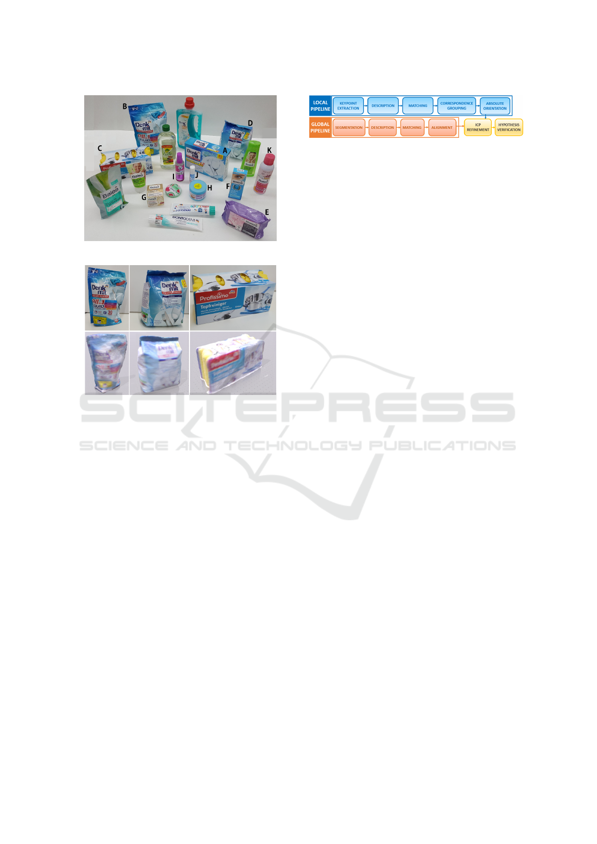
Figure 2: Object training set.
Figure 3: Some reconstructed 3D models.
not labelled in Figure 2). All the models are finally
converted into Point Cloud Data (.pcd) files, to be
elaborated by the Point Cloud Library (PCL) (Rusu
and Cousins, 2011). A complete point cloud model
could have regions that are doubled in overlapping ar-
eas, due to small registration errors, and holes, due
to scanning surfaces that did not return any distance
measurements (e.g., shiny or metallic objects). There-
fore, the obtained point clouds are then filtered with
the Moving Least Squares (MLS), which is a widely
used technique for approximating scattered data us-
ing smooth functions.
2.3 Comparison Among Existing
Algorithms
One of the main goals of 3D data processing is about
matching regions. This process generally happens
between two point sets S
1
and S
2
, which can be
compared through a method based on the descrip-
tor notion. Descriptors can be defined like the struc-
tures that contain useful information to summarize the
points of a point cloud and in this work they are used
to search correspondences between an object model
and scene points. As described in (Aldoma et al.,
2012), depending on the way they represent the infor-
Figure 4: The SoA local and global pipelines.
mation, 3D descriptors can be divided into two main
categories: Signatures or Histograms. The descrip-
tor of each category, depending on the extension of
the point cloud to which it is applied, can be local or
global. Descriptors of single objects and scene areas
belong to the local category, while global descriptors
describe the scene using all pixels of the image. On
this distinction, the state of the art advises to follow
two possible pipelines, depending on the case study,
shown in Figure 4. However, many limitations have
been found to generalize the recognition and localiza-
tion tasks and that is why a new hybrid approach has
been adopted.
2.3.1 Local Pipeline
3D local descriptors work on specific points, called
keypoints. They contain information from a neighbor-
hood, which is usually determined by selecting points
within a radius from the center point. The descrip-
tion of a complete object consists in associating each
point with a descriptor of the local geometry of the
same point. Referring to Figure 4, the main phases of
a local pipeline are the first three:
1. Keypoint Extraction: They represent points
of interest which are stable, characteristic or distinc-
tive. However, tests carried out with extracted edges,
a typical keypoint criterion, did not produce satisfac-
tory results in cluttered scenes.
2. Description: This second step associates the
descriptors to the keypoints. As above, a common
trait of all local descriptors is the definition of a local
support used to determine the subset of neighboring
points around each keypoint that will be used to com-
pute its description: the best choice for the support
size was about 0.02m. Intuitively, it is understood
how the support size may be defined either in terms
of length, or in terms of the number of neighbors.
During experimental tests, the choice has been obvi-
ously a trade-off since a fixed number of neighbors
means that histograms will have the same total magni-
tude but will also be more susceptible to differences in
point density. This means that the radius parameter is
somewhat robust but its size does need to be tuned for
the specific class of object that is being recognized: if
the size is too small, the descriptor will describe basic
features like planes and corners and will lose its abil-
ity to discriminate. On the other hand, if the radius is
too large it will contain information from much of the
ICINCO 2018 - 15th International Conference on Informatics in Control, Automation and Robotics
112

background and it will not match to anything.
3. Matching: Then, a pair of points (p
m
, p
s
),
with p
m
point of the model and p
s
point of the
scene, can be defined a correspondence if their Eu-
clidean distance is below a certain threshold, chosen
a priori by the user. To make the comparison step
even more efficient, it has been applied a particular
comparison pattern on the matching neighborhoods
found, called the Fast Library Approximate Near-
est Neighbors (FLANN) algorithm (Muja and Lowe,
2009). Even in this step, searching the optimal thresh-
old value is crucial: a too low value generates too
many possible combinations in the total scene; a too
high value makes the matching algorithm too greedy.
Searching a unique value for different scenes and the
same model was impossible.
2.3.2 Global Pipeline
Global descriptors are high-dimensional representa-
tions of the geometric features of an object. Their use
is similar to that of local descriptors but, due to high
computational cost, they are generally calculated af-
ter a 3D segmentation. Even if the global sequence of
phases is similar to that of the local pipeline, there is a
deep difference: the object is now described in its en-
tirety and not only through some of its points, without
keypoints. With reference to Figure 4, the main steps
of a global pipeline are:
1. Segmentation: Segmentation is a well-
researched topic and several techniques exist
(Bergstrom et al., 2011), (Mishra and Aloimonos,
2011), (Comaniciu and Meer, 2002). It is needed
to identify the various objects that are part of the
scene. Different techniques can be used, such as
the Differences between point clouds, which is
a background subtraction method, the Euclidean
pooling method that splits point clouds in a series of
subgroups distant among each other a given amount
(similar to the k-mean segmentation), Extraction of
polygons and solids, which detects a subset of points
that resemble a geometrical primitive (cylinder,
sphere, ...), Segmentation of normal method, based
on the extraction of surfaces whose normals have a
particular direction.
2. Description: The output of scene segmenta-
tion is a set of clusters, supposedly each representing
a single object of the scene. The shape and geometry
of each of these objects are described by means of a
proper global descriptor and represented by a single
histogram. It is obvious that the obtained descriptor
is highly affected by partial occlusions, hence the fol-
lowing matching phase will likely fail in such cases.
3. Matching: In all cases, the histogram is in-
dependently compared against those obtained in the
Figure 5: The proposed hybrid pipeline.
training stage, getting the best N matches. Matches
are not pairs of points as in the case of local descrip-
tors, but the set of N model views that can be su-
perimposed on the scene by applying a transforma-
tion. Typically, the histogram matching is done using
FLANN by means of a brute force search, and the dis-
tance between histograms is computed using the L
1
metric.
2.3.3 Hybrid Pipeline
Taking into account that, in the considered applica-
tion, only geometric information about the objects
is available (no visual features are used), the scene
is usually large and affected by partial occlusions,
similar objects are close to each other, local and
global SoA pipelines are not suitable for the limita-
tions discussed above. The proposed algorithm ex-
tracts the most generalizable steps of each standard
SoA pipeline, that means the global segmentation and
the local descriptor robustness, as shown in Figure 5.
Moreover, a new approach is introduced: unlike the
SoA pipeline that provides the matching phase and the
alignment phase as two separated steps, the proposed
algorithm takes the two phases in one step. It also
optimizes a critical parameter to be more efficient and
robust than the traditional approach. The initial coarse
alignment provided by the RANdom SAmple Con-
sensus (RANSAC) method (Papazov and Burschka,
2011) is finally refined by the Iterative Closest Point
(ICP) method (Rusinkiewicz and Levoy, 2001). The
output of the proposed algorithm is the 6D pose of the
recognized object. The hybrid pipeline is divided into
8 steps:
1. PassThrough Filtering. A series of filters
available in the PCL library are applied to the input
point cloud in order to reduce undesirable data. Since
the objects are all placed on a flat surface of known
size and location, it is easy to identify the portion of
the scene of interest and remove the rest.
2. Plane Segmentation. The segmentation of
normal method, cited in the global pipeline, has been
chosen because in the supermarket scenario objects to
pick are placed on trolley trays. PCL provides a very
useful component to perform this task, called Sample
Consensus Segmentation. This component is based
on the RANSAC method, which is a randomized al-
gorithm for robust model fitting. It is used to esti-
Flexible Motion Planning for Object Manipulation in Cluttered Scenes
113
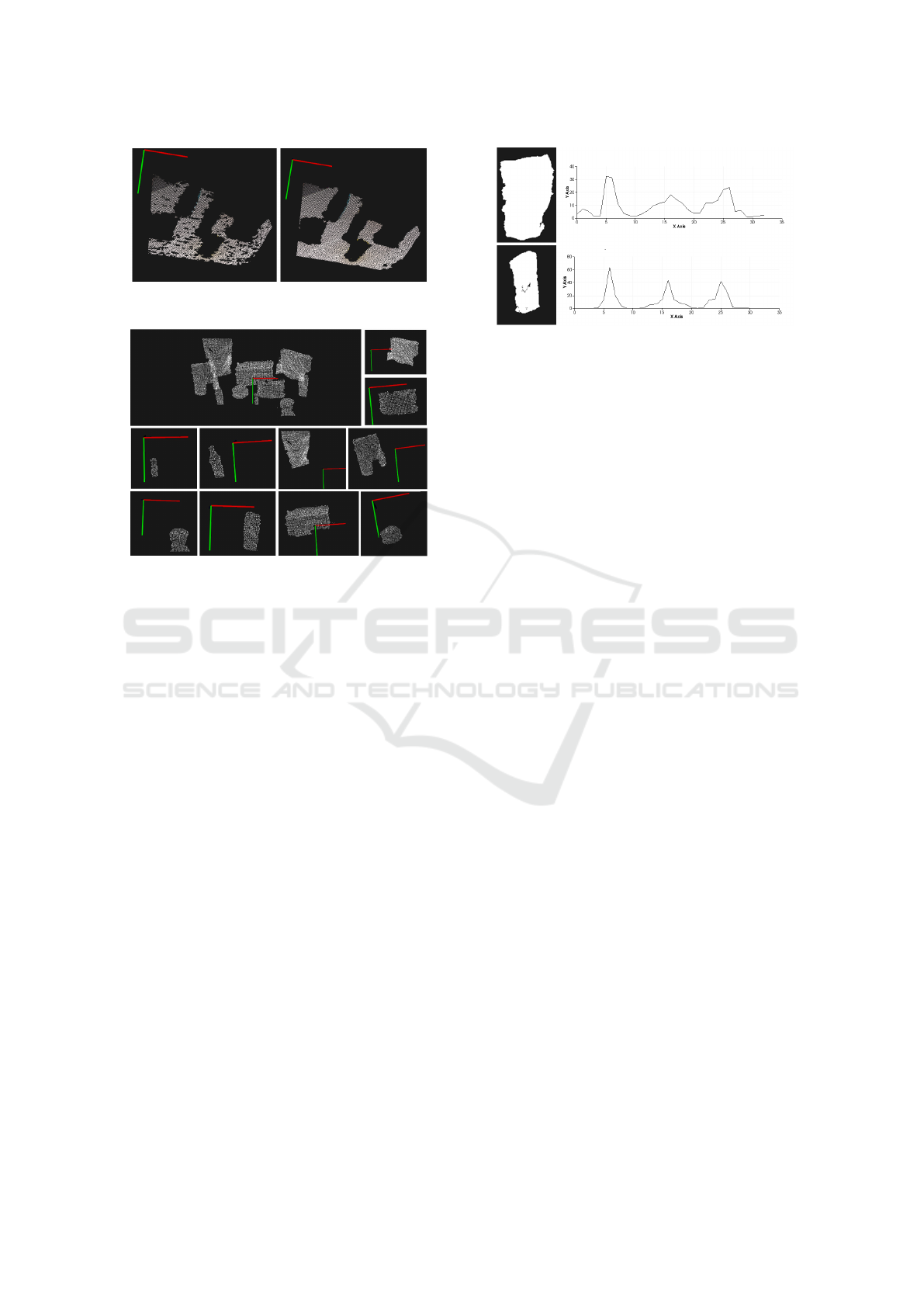
Figure 6: k dependence for the plane segmentation. (a) k=5;
(b) k=100.
Figure 7: Clustering process.
mate parameters of a mathematical model from a set
of observed data that contain both inliers (those points
satisfying the model condition) and outliers (all other
points). The output of this segmentation process is a
vector of model coefficients, which are used to show
the contents of the inlier set. Note that extracting the
plane strongly depends on the quality of the surface
normals, as shown in Figure 6. The image on top-left
of Figure 7 illustrates the outcome of this step.
3. Objects clustering. The final step of the seg-
mentation process is the clustering, that means cat-
egorize objects of the scene. The task uses the Eu-
clidean Cluster Extraction approach: assuming that a
Kd-tree structure is used for finding the nearest neigh-
bors, it is needed to fix a threshold d
t
, which indi-
cates how close two points are required to belong to
the same object. By selecting d
t
, the clusters reported
in Figure 7 are obtained from the scene.
4. Data Pre-processing. Before the descriptor
analysis, as already done for the object models, each
cluster is passed through the MLS filter, to improve
the quality of the geometric descriptor.
5. VoxelGrid Filter Downsampling. To apply
the local FPFH descriptor, a simple downsampling
step through a Voxelized Grid approach has been used
as a keypoint extraction method. Because model and
scene can be provided by different data sources, as
seen in Section 2.2, this step makes them more sim-
ilar and improves the consistency between the model
descriptor of an object and the descriptor of the re-
Figure 8: FPFH descriptors of two objects in the set.
spective cluster, by providing a priori knowledge of
the point cloud density. Furthermore, downsampling
reduces computational cost.
6. FPFH Descriptors. Several experiments with
different descriptors have been carried out and the
FPFH local descriptor has been selected for its robust-
ness. Global descriptors like VFH, ESF or PFH have
been analyzed but everyone suffers from some of the
specific application requirements. Although the per-
formance of these global descriptors, in ideal oper-
ating conditions as described by their authors, repre-
sents a good solution to solve the object recognition
problem, the following factors have led to the selec-
tion of a local descriptor:
• the scenarios are complex in the sense that they
contain many objects also similar to each other;
• the objects can be distant from the camera up to
two times the ideal distance of 0.5 m defined in
the ideal operating conditions (see Section 2.3.4);
• the objects are very often occluded;
FPFH features represent the surface normals and the
curvature of the objects, as shown in Figure 8.
7. Point clouds initial alignment: OPRANSAC.
Given two generic S
source
and S
target
point clouds in
3D space, to be compared they need to be aligned, that
means to calculate the rigid geometric transformation
to be applied to S
source
to align it to S
target
. In this
work, an initial alignment is obtained by following
the approach in (Buch et al., 2013), i.e., the Prerejec-
tive RANSAC. This method uses the local FPFH de-
scriptors as the parameters of the consensus function,
it finds inliers points and finally it provides the es-
timated geometric transformation. This alignment is
calculated without having previous knowledge about
the position or orientation of the target object. To
setup the alignment process, the class SampleConsen-
susPrerejective has been used, which implements an
efficient RANSAC pose estimation loop.
The following difficulties have been encountered
during this phase: in some similar scenes in which the
objects on the table were slightly moved, the SoA al-
ICINCO 2018 - 15th International Conference on Informatics in Control, Automation and Robotics
114
gorithm did not correctly recognize the model object,
often confusing it with objects of different geometry.
When it recognized the model, the correspondence
rates were very different from one scene to another or
similar for different objects. So, the results obtained
by these common techniques did not meet the super-
market scenario requirements. This is why a careful
analysis of this crucial step has been carried out in or-
der to identify only the most sensitive parameters that
affect the algorithm result. The critical parameter that
has been identified is the number of nearest features
to use (γ): small changes generate very different out-
puts. Then, the objective was to try to select a single
value of this parameter for every observed scene and
for every object model but all attempts were vain. The
adopted solution is to maximize the following fitness
function over γ:
[I, H] = RANSAC(S
source
,S
target
,γ) (1)
f itness(γ) =
|I|
|S
source
|
, (2)
where |I| is the cardinality of the set I of inliers
points between the two point clouds S
target
and S
source
after the RANSAC alignment calculated by using the
current value of γ, and H is the 4 × 4 homogenous
transformation matrix to perform such alignment.
In order to maximize the fitness function, two
nested loops have been implemented. The inner one
computes the best γ variable by increasing it each time
of a fixed step (i.e., δ
γ
= 5). The external one ex-
ecutes this operation for each target cluster S
target
[ j]
labelled in the specific scene, i.e., with j from 1 to the
number of clusters identified in the scene. Finally, the
best result is chosen: the corresponding homogenous
transformation matrix and the labelled cluster are se-
lected. This approach has provided surprising and ro-
bust results and it has been called OPRANSAC to un-
derline the optimization process. The pseudo-code is
reported in Algorithm 1.
The maximum fitness value, equal to 1, is obtained
when all the points have a near distance below the
fixed δ
th
threshold. The partiality of the views (clus-
ters) and therefore of the point clouds makes unlikely
an high level of fitness, although over 70% of match-
ing in the experimental tests have been found. The
definition of the similarity parameter therefore allows
to compare incomplete objects and models but also it
allows to define an optimization heuristics based on
the cardinality of the point clouds. Figure 9 shows
some results.
8. ICP. Finally, the ICP algorithm is applied to
refine the estimated 6-DoF object pose. Figure 10 il-
lustrates its output.
Algorithm 1: OPRANSAC initial alignment.
1: input:
2: S
source
← model point cloud to identify
3: S
target
← vector of all labelled clusters
4: γ
0
← initial value of the critical parameter γ
5: N ← number of iteration for internal loop
6: δ
γ
← fixed step for the critical parameter
7: procedure PERFORM ALIGNMENT
8: f itness = 0
9: H = I
4×4
10: label = 0
11: for j = 1 to S
target
.size do
12: γ = γ
0
13: for i = 1 to N do
14: [I, H
temp
] = RANSAC(S
source
,S
target
[ j],γ)
15: f itness
temp
= |I|/|S
source
|
16: if f itness
temp
> f itness then
17: f itness = f itness
temp
18: H = H
temp
19: label = j
20: γ+ = δ
γ
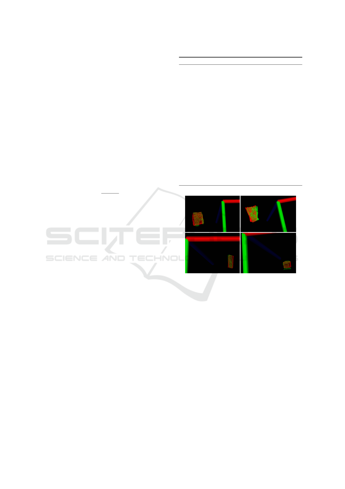
Figure 9: Coarse alignment: cluster (green) and
OPRANSAC result (red).
2.3.4 Tests and Performance Assessment
In this subsection the most interesting results obtained
by testing the proposed algorithm will be discussed.
Camera Placement. Camera placement depends
on three factors. Camera height influences both plane
segmentation and object clustering processes. The
higher it is placed, the better is the plane segmen-
tation, however the worse is the object clustering.
Camera distance from the scene affects the dimen-
sions of the clusters and the dimensions of the cap-
tured scene. The larger is the distance, the smaller are
the object clusters and the corresponding point clouds
have fewer points. On the other hand, to frame as
many objects as possible the distance should be large
enough. Finally, the distance should high enough to
let the camera stay out of the robot workspace so as
to avoid an additional obstacle for the pick and place
process. As a trade off among the discussed factors,
Flexible Motion Planning for Object Manipulation in Cluttered Scenes
115
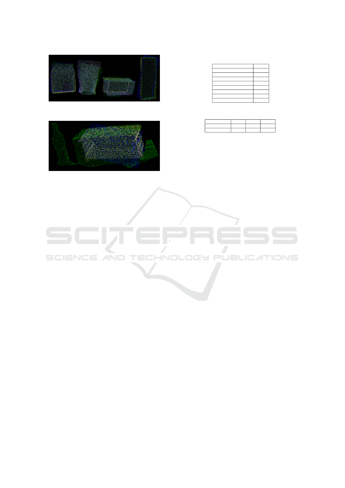
Figure 10: Refined alignment: ICP (yellow) adjusts the
OPRANSAC (blue) alignment on the cluster (green).
Figure 11: Good alignment with an incorrect clustering (ob-
jects too close).
the best distance range of the camera with respect to
the objects is between 0.30m and 0.90m.
Object Placement. Other relevant aspects are the
distance among objects and their placement on the
tray. In this work objects are assumed to be randomly
placed but all upright on the tray and at a minimum
distance of 0.3 m, which is quite critical for a success-
ful collision free motion planning of the grasp phase
(see Section 3.2). However, tests with shorter dis-
tances have been demonstrated that the recognition
phase has still good results as in the example shown
in Figure 11, where a cluster erroneously contains two
objects but the OPRANSAC alignment algorithm cor-
rectly aligns the model to the right part of the cluster.
Analysis of the Execution Time. Several experi-
ments have been done to measure the execution times
and to evaluate the performance of the recognition al-
gorithm. Table 1 shows the main parameters settings.
Then the execution time of the two main phases of the
algorithm is calculated, based on an observed scene
containing 11 objects. The data, expressed in seconds,
are reported in Table 2. Note that the OPRANSAC
step requires more computational time due to the in-
troduction of the N-loop for each cluster. The refine-
ment ICP phase shows a constant trend around 700
milliseconds, which is irrelevant.
Confusion Matrix. To evaluate the behavior of
the proposed algorithm in terms of its precision and
reliability during the object classification, an exten-
sive test has been executed, where the known objects
are randomly placed on a tray as explained above.
The confusion matrix (Table 3) related to twenty dif-
ferent scenes shows the recognition rate of the pro-
posed algorithm. It is important to remark that with-
Table 1: Alignment parameters settings.
OPRANSAC
ransac_max_iter 50000
ransac_inlier_fraction 0.25
ransac_num_samples 3
ransac_similarity_thresh 0.9
ICP
icp_max_corr 0.01
icp_out_thresh 0.01
icp_max_iter 50000
Table 2: Execution times (in seconds).
min max mean
OPRANSAC 31.25 134.7 75.7
ICP 0.5 1.4 0.7
out a criterion to exclude uncertain recognitions, ob-
jects are always recognized and this can produce a
high value of false positives. A simple way to reduce
this phenomenon is to fix a threshold, δ
f it
, to exclude
the cases of poor likeness. This alternative method
improves also the execution time of the algorithm be-
cause the expected loop is interrupted if the average
model-cluster correspondence is lower than δ
f it
. For
each test, the algorithm is invoked, taking the model
of the object to be recognized as input. The algorithm
output is a selected cluster with a fitness value, fit-
ness. By comparing fitness with δ
f it
, it is possible to
choose if the correspondence is acceptable or not: if
f itness > δ
f it
, the model-cluster association is con-
sidered valid (1), otherwise no (0). Table 3 reports
the percentage results by repeating this test for all ob-
ject models in the same scene and for twenty different
scenes. The values in the last column correspond to
the cases of failed recognition ( f itness < δ
f it
).
The C, D, F boxes have a higher number of hits be-
cause their fitness match values are always the high-
est for their respective clusters than that with the other
clusters, and so the percentage of failure when the aim
is to recognize these objects is low. However, they
are the objects with simpler geometry and large sur-
face extension, and this means that their point clouds
clusters have obviously more samples than those of
the others objects. On the opposite side, the clusters
of the G, H, I, J objects have fewer points because
they are small items and also their distance from the
camera cause very coarse and distorted clusters. This
limits the fitness values and therefore the success of
the algorithm. The curvatures of the smaller objects
are not well defined in the clusters and even the fil-
tering is not enough to represent them better. So, the
result is a low fitness value implying that the desired
model is often confused with an incorrect cluster.
By aggregating the data, 220 tests have been car-
ried out: the algorithm has produces 156 true positive
and 52 false positives, which correspond to a correct
recognition in the 71% of cases and a wrong recog-
nition in the remaining 23%: the remaining 6% of
ICINCO 2018 - 15th International Conference on Informatics in Control, Automation and Robotics
116
Table 3: Confusion matrix based on 20 observed scenes
(recognition rate%): models (capital letter) and clusters
(lowercase letter) as labelled in Figure 2. UR indicates un-
recognition rates.
a b c d e f g h i j k UR
A 50 10 20 20 0 0 0 0 0 0 0 0
B 0 90 0 0 0 10 0 0 0 0 0 0
C 0 0 100 0 0 0 0 0 0 0 0 0
D 0 0 0 100 0 0 0 0 0 0 0 0
E 0 0 0 0 60 0 30 10 0 0 0 0
F 0 0 0 0 0 100 0 0 0 0 0 0
G 0 0 0 0 0 0 60 40 0 0 0 0
H 0 0 0 0 0 0 20 70 0 0 0 10
I 0 0 0 0 0 20 0 10 60 0 0 10
J 0 0 0 0 0 0 0 0 40 30 0 30
K 0 0 0 0 0 0 0 0 0 30 60 10
the cases analyzed did not produce any association at
least equal to δ
f it
.
3 FLEXIBLE MOTION
PLANNING
Enabling a robot manipulator to have the perception
of its workspace can drastically improve the flexibil-
ity of a industrial system. In this context, this work
aims not only to design a 3D vision system able to
identify the desired object pose, but also a reliable
control able to manipulate it in a dynamic scene. The
accuracy has to be sufficient to move the object into
the robot workspace without causing issues such as
damage or errors. This section describes how two
main problems have been solved: the planning of
unnecessary robot reconfigurations, and the on-line
collision avoidance with unexpected and uncertainly
placed objects. The first problem has been solved in-
tegrating the Stochastic Trajectory Optimization for
Motion Planning (STOMP) planner and the Trac-IK
kinematics solver into the MoveIt! framework used
for motion planning. The second problem has been
solved with a reactive control strategy based on dis-
tributed proximity sensors used to compute in real-
time a modification of the planned trajectory to avoid
collisions with unexpected objects in the scene.
3.1 Sensory System
The optimal placement of the RealSense camera
for the localization and recognition task (see Sec-
tion 2.3.4) did not allow to frame the whole robot
workspace. Thus, a second depth camera, the Mi-
crosoft Kinect, after the calibration procedure already
described in Section 2.1, has been integrated into the
MoveIt! architecture to build the 3D scene recon-
struction for robot motion planning.
To better avoid collisions during the robot planned
trajectories, e.g., with objects not known or not per-
fectly modeled in the scene, four proximity sensors
have been mounted on the gripper (see Figure 14),
along four main directions (top, bottom, right, left).
They have been connected to the Arduino Mega
2560 micro-controller through a TinkerKit shield con-
nected to the ROS network via a serial interface.
3.2 Motion Planning Pipeline
Humans use a remarkable set of strategies to manip-
ulate objects, especially in complex scenes. They
pick up, push, slide, and sweep objects with their
hands and arms to rearrange surrounding clutter. But
the robots look the world differently: they move ob-
jects through pick-and-place actions, typically grasp-
ing objects in fixed points. The aim of this subsection
is to develop a smart pipeline for the robotic manipu-
lation planning based on heuristic considerations.
IK Constrained Solution. Trac-IK Solver is
an inverse kinematics solver developed by Traclabs
that achieves more reliable solutions than commonly
available open source IK solvers (Beeson and Ames,
2015). It provides an alternative inverse kinemat-
ics solver to the MoveIt! interface and replaces the
default KDL solver. During the experimental tests,
KDL algorithms, based on Newton’s method, had
convergence problems due to the presence of joint
limits. Instead, Trac-IK merges a simple extension
to KDL’s Newton-based convergence algorithm, that
detects and mitigates local minima due to joint limits
by random jumps, and a Sequential Quadratic Pro-
gramming (SQP) constrained nonlinear optimization
approach, which uses quasi-Newton methods that bet-
ter handle joint limits. By default, the IK search re-
turns immediately when either of these algorithms
converges to an answer. For this work, secondary con-
straints of manipulability are also provided in order
to obtain the ‘best’ IK solution. To avoid unneces-
sary reconfigurations, virtual joint limits on relevant
joints (see Section 4 for more details) have been used
to compute the target configuration to keep it as close
as possible to the starting configuration.
STOMP Planner. To choose which planner to
use, both the planning time and the quality of the
trajectories have been analyzed in detail. First of
all the default MoveIt! Open Motion Planning Li-
brary (OMPL) has been considered. OMPL pro-
vides eleven motion planning algorithms, many of
which implement different SoA methods (Kalakrish-
nan et al., 2011). All these planners have been
tested, by studying the significant parameters and
tuning their values. Some planners are quite slow,
while some others are unable to provide a solution.
The table in Figure 12a shows the results: only
Flexible Motion Planning for Object Manipulation in Cluttered Scenes
117

Figure 12: Typical OMPL planned path Vs STOMP solu-
tion.
five of them provided a solution in complex scenar-
ios. In particular, only three planners (RRTConnec-
tkConfigDefault, RRTkConfigdefault and BKPieceK-
ConfigDefault) gave good solutions in the shortest
planning time.
The conclusion of these tests is that OMPL pro-
vides consistent theoretical algorithms but difficult
to tune and use effectively in practice. The idea
of having a limited number of parameters, which
the user is called to define to configure the chosen
method, implies that the motion planning manage-
ment is fully centralized in the algorithm itself and
determined by the user in a small part. In these terms,
on the one hand this is an advantage but, in practice,
the strong stochastic nature of sample-based motion
planners has been unsatisfactory because the plan-
ners often elaborate unnatural trajectories, as the red
planned trajectory in Figure 12b shows. For this rea-
son, a more recent optimal planning algorithm, called
STOMP (Kalakrishnan et al., 2011), has been inte-
grated. After hundreds of tests carried out in differ-
ent environments, the conclusion is that in complex
scenes, the STOMP motion planner presents a little
longer response time to plan a path, but returns the
best natural and smooth trajectories, far enough from
the obstacles.
Obstacle Avoidance. The Kinect camera frames
the real-time changes of the scene and sends these in-
formation to MoveIt! that updates the ROS environ-
ment. There are some ROS drivers available to in-
tegrate this camera with ROS: this system uses the
openni_kinect driver, which provides point clouds.
The camera is fixed in such a way to cover the robot
worksapace as in Figure 1. Figure 13a shows how
MoveIt! takes the Kinect depth map as input and
publishes a filtered cloud into its RViz environment.
This filtered cloud includes the environment around
the robot except the robot kinematic chain and every-
thing described as ‘collidable’ object into the URDF
file. The problem is that MoveIt! cannot consider
the appearing objects in the scene as obstacles only
through the point cloud. For this purpose, it is nec-
essary to create the 3D Occupancy Map as shown in
Figure 13b. The Octomap provides the 3D models in
Figure 13: (a)Point cloud into ROS environment; (b) Oc-
toMap.
the form of volumetric representation of the space and
lets the motion planner plans the collision free path.
It is a 3D occupancy grid map, based on the octree
structure (Hornung et al., 2013).
Among the MoveIt! capabilities, the collision de-
tection is solved through a default collision checking
library, called Flexible Collision Library (FCL). FCL
supports collision checking for various object types,
e.g., OctoMap (Pan et al., 2012).
Task Planning. The implementation of the super-
market scenario task reveals some difficulties, such
as:
• the motion planner must have exact knowledge
about the robot and its environment;
• every collision that could harm the robot and the
environment itself has to be avoided but other col-
lisions are necessary, e.g., when the robot has to
get in contact with the graspable object;
• the grasped object has to be considered as an ad-
ditional part of the robot, hence it should be in-
cluded in the robot kinematic chain during the
motion planning because it possibly increases the
size of the end effector;
• it is possible to have additional constraints, such
as carrying bottles filled with liquid in an upright
position.
A temporal segmentation of the whole task can be a
simple solution:
1. Pre-grasp Phase. The robot moves from its cur-
rent configuration to the grasp point neighbor-
hood.
2. Grasp Phase. The robot grasps the object.
3. Manipulation Phase. The grasped object is
raised a few centimeters from its support plane
and finally moved till the target point neighbor-
hood.
4. Release Phase. The robot reaches the goal loca-
tion and releases the object.
5. Retreat Phase. The robot retreats from the ob-
ject.
ICINCO 2018 - 15th International Conference on Informatics in Control, Automation and Robotics
118

Figure 14: Gripper with proximity sensors (red arrows are
the z axes of the sensor frames).
For each subtask, starting from the robot current con-
figuration and given the target pose, the IK is solved
by the TracIK solver, which returns to STOMP the
target configuration. Finally, STOMP off-line plans
the desired trajectory in the joint space, that is q
d
(t).
3.3 Reactive Control
Even though the planned arm path is collision-free,
the uncertainties on the object locations and the pos-
sibility of unseen subjects could lead to unexpected
collisions. To counteract these issues, a real-time re-
active control algorithm is used at execution time to
adapt the planned motion to the actual scene. The
method is based on the well-known artificial poten-
tial approach (Khatib, 1986) and further developed
in (Falco and Natale, 2014) for a mobile manipulator.
The planned motion in the joint space q
d
(t) is modi-
fied on the basis of the distances d
i
,i = 1,.. .,4 com-
puted by the four proximity sensors mounted on the
gripper as shown in Figure 14. A frame Σ
i
is attached
to the ith sensor, with an orientation with respect to
the robot base frame represented by the rotation ma-
trix R
si
(q), where q is the current robot configuration.
Then a virtual repulsive force applied to the ith sensor
is computed as
f
si
i
=
[
0 0 −α/d
i
]
T
if d
mi
< d
i
< d
Mi
[
0 0 0
]
T
otherwise
(3)
being α a suitable gain and d
mi
and d
Mi
two thresholds
defining the distance range within which the reactive
control is active. This repulsive force is then trans-
lated into a joint displacement as
δq = β
4
∑
i=1
J
T
i
(q)R
si
f
si
i
, (4)
where J
i
(q) is the arm jacobian computed until the ith
sensor frame and β is a gain (with the dimensions of
a rotational compliance) translating the virtual elas-
tic joint torque J
T
i
(q)R
si
f
si
i
into a joint displacement.
Finally, such displacement is simply added to the
planned motion q
d
(t), thus endowing the robot with
the capability to react to scene uncertainties and dy-
namics as demonstrated by the experiment presented
in the next section.
4 EXPERIMENT
This section describes the execution of a fetch and
carry task typical of a shelf refilling process in a su-
permarket. The robot workspace is shown in Figure 1,
with a table and some objects to grasp. Under the as-
sumptions specified in Section 2.2, they are randomly
located on the plane and their positions and orienta-
tions are not known. The goal of the considered task
is to place two objects (labelled as F and K in Fig-
ure 2) on the shelving unit, by fixing a target pose
very close to other objects already present.
Object Recognition and Localization. After
preparing the scene, it is possible to select the spe-
cific object to grab. There are two main steps. First of
all, an instantaneous frame of the RealSense scene is
saved in the form of point cloud. Then, the hybrid
pipeline proposed in Section 2.3.3 is called to rec-
ognize a specific object, starting from its point cloud
model. The algorithm provides the object pose with
respect to the robot base represented by the T
base
grasp
ho-
mogenous transformation matrix.
Off-line Trajectory Planning. The T
base
grasp
matrix
is used to define the picking pose of the end effec-
tor. The planning pipeline described in Section 3.2
is sequentially executed. The STOMP planner is in-
voked at every step. It generates a trajectory by con-
sidering the robot current configuration and the target
configuration provided by the IK solver. The Trac-IK
solver finds a solution which has to be collision-free.
If the target pose corresponds to an unreachable or
colliding pose, the solver gives up and the task is in-
terrupted. During the tests, the S, E and T joints (see
Figure 1) have been identified as the most critical for
the robot reconfiguration problem. Two sets of virtual
joint limits, one with positive ranges for the selected
joint angles and the other negative, have been defined.
The IK solver chooses between the two sets according
to the signs of the selected joints in the robot current
configuration, thus trying to avoid a reconfiguration,
e.g., from elbow up to elbow down.
Reactive Control. Octomap has proved to be a
rough method to plan collision-free trajectories for
tasks that require high accuracy and responsiveness.
Unfortunately, it cannot be sufficient. In this exper-
iment, some objects are placed on the shelving unit
and the robot is asked to place the grasped object in
Flexible Motion Planning for Object Manipulation in Cluttered Scenes
119
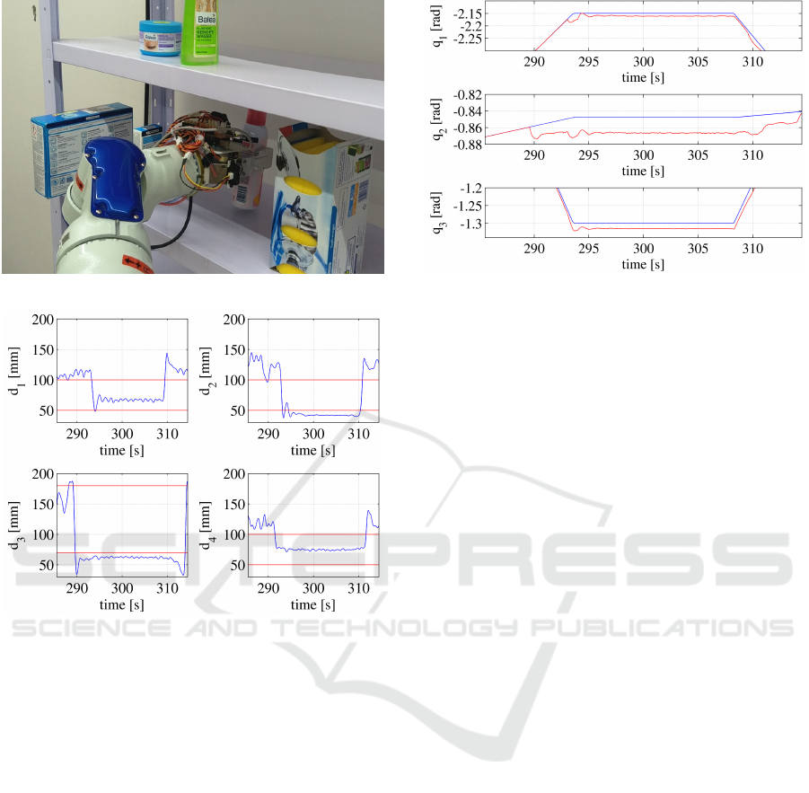
Figure 15: Local trajectory adjustment: place phase.
Figure 16: Distances measured by the proximity sensors
during the place subtask (thresholds in red).
a position very close to them. The Kinect accuracy
is not enough to satisfy the required precision. The
use of the proximity sensors can locally correct the
planned trajectory, in order to better place the objects.
According to this task, the proximity sensors thresh-
olds in (3) are set as follows:
• d
m
i
= 50mm, d
M
i
= 100mm, i=1,2,4
• d
m
3
= 70mm, d
M
3
= 170mm
while the gains are α = 5 Nmm and β = 0.3 rad/Nm.
The use of proximity sensors has proved to be fun-
damental during the place phase. As shown in Fig-
ure 15 and in the distance signals reported in Fig-
ure 16, when the robot end effector enters the shelv-
ing unit, the 3rd proximity sensor (with reference to
the numbers in Figure 14) detects the upper edge of
the shelf, which produces a repulsive downward force
applied to the end effector computed as in (3). This
force is transformed into joints displacement δq and
added to the planned configuration q
d
(t) until the spe-
cific sensor reads distances into the reactive range, as
shown in Figure 17, which reports some planned and
Figure 17: Planned (blue) and actual (red) positions of the
first three arm joints.
actual joint positions. Then, the 2nd sensor detects
the presence of an obstacle, which produces a repul-
sive rightward force applied to the end effector. From
this moment, the joints displacement δq overlaps the
effects of both sensors. Subsequently, the end effector
tries to reach the deep target pose following the mod-
ified planned trajectory. Thus, even the right object is
detected by the 1st sensor. As before, a new repulsive
force is generated and the combination of the other
two produces a new displacement. In this way, the
grasped object is safely placed on the shelf. A video
of the complete experiment can be found at the link:
https://www.dropbox.com/s/3817sotnno70khp
/clip.mp4?dl=0.
5 CONCLUSIONS
This paper presented the implementation of a com-
plete fetch and carry task typical of the in-store logis-
tic scenario, where a large number of different items
have to be handled. The proposed methods range
from object recognition and localization in cluttered
scenes to motion planning and reactive control. El-
ements of novelty have been proposed in all these
technologies that revealed essential for a successful
execution of the task in a real setting. Limitations of
the approach are mainly due to the perception sys-
tem for object recognition. The objects are required
to be placed at a certain distance from each other and
no transparent or thin or polished objects can be han-
dled as it is difficult to reconstruct a good quality point
cloud in such cases. Future work will be devoted to
integrate the approach with the slipping control strat-
egy by (Costanzo et al., 2018), which aims at enhanc-
ing robustness of the task execution.
ICINCO 2018 - 15th International Conference on Informatics in Control, Automation and Robotics
120

ACKNOWLEDGEMENTS
This work was supported by the European Commis-
sion within the H2020 REFILLS project ID n. 731590
and the H2020 LABOR project ID n. 785419.
REFERENCES
Aldoma, A., Marton, Z.-C., Tombari, F., Wohlkinger, W.,
Potthast, C., Zeisl, B., Rusu, R., Gedikli, S., and
Vincze, M. (2012). Tutorial: Point cloud library:
Three-dimensional object recognition and 6 DOF pose
estimation. IEEE Robotics & Automation Magazine,
19(3):80–91.
Beeson, P. and Ames, B. (2015). TRAC-IK: An open-
source library for improved solving of generic inverse
kinematics. In 2015 IEEE-RAS 15th International
Conference on Humanoid Robots (Humanoids), pages
928–935. IEEE.
Bergstrom, N., Bjorkman, M., and Kragic, D. (2011). Gen-
erating object hypotheses in natural scenes through
human-robot interaction. In 2011 IEEE/RSJ Interna-
tional Conference on Intelligent Robots and Systems,
pages 827–833. IEEE.
Buch, A. G., Kraft, D., Kamarainen, J.-K., Petersen, H. G.,
and Kruger, N. (2013). Pose estimation using local
structure-specific shape and appearance context. In
2013 IEEE International Conference on Robotics and
Automation, pages 2080–2087. IEEE.
Comaniciu, D. and Meer, P. (2002). Mean shift: A robust
approach toward feature space analysis. IEEE Trans-
actions on Pattern Analysis and Machine Intelligence,
24:603–619.
Costanzo, M., De Maria, G., and Natale, C. (2018). Slip-
ping control algorithms for object manipulation with
sensorized parallel grippers. In 2018 IEEE Interna-
tional Conference on Robotics and Automation. IEEE.
Falco, P. and Natale, C. (2014). Low-level flexible planning
for mobile manipulators: a distributed perception ap-
proach. Advanced Robotics, 28:1431–1444.
Hornung, A., Wurm, K. M., Bennewitz, M., Stachniss, C.,
and Burgard, W. (2013). OctoMap: An efficient prob-
abilistic 3D mapping framework based on octrees. Au-
tonomous Robots, 34:189–206. Software available at
http://octomap.github.com.
Kalakrishnan, M., Chitta, S., Theodorou, E., Pastor, P., and
Schaal, S. (2011). STOMP: Stochastic trajectory opti-
mization for motion planning. In 2011 IEEE Interna-
tional Conference on Robotics and Automation, pages
4569–4574. IEEE.
Kavraki, L., Svestka, P., Latombe, J.-C., and Overmars, M.
(1996). Probabilistic roadmaps for path planning in
high-dimensional configuration spaces. IEEE Trans-
actions on Robotics and Automation, 12(4):566–580.
Khatib, O. (1986). Real-time obstacle avoidance for manip-
ulators and mobile robots. Int. J. Rob. Res., 5:90–98.
Khokar, K., Beeson, P., and Burridge, R. (2015). Imple-
mentation of KDL inverse kinematics routine on the
atlas humanoid robot. Procedia Computer Science,
46:1441–1448.
Kuffner, J. and LaValle, S. (2000). RRT-connect: An effi-
cient approach to single-query path planning. In Pro-
ceedings 2000 ICRA. Millennium Conference. IEEE
International Conference on Robotics and Automa-
tion. Symposia Proceedings (Cat. No.00CH37065),
pages 995–1001. IEEE.
Mishra, A. and Aloimonos, Y. (2011). Visual segmentation
of simple objects for robots. In Robotics: Science and
Systems VII, pages 1–8. Robotics: Science and Sys-
tems Foundation.
Muja, M. and Lowe, D. G. (2009). Fast approximate near-
est neighbors with automatic algorithm configuration.
In In VISAPP International Conference on Computer
Vision Theory and Applications, pages 331–340.
Nakhaeinia, D., Payeur, P., and Laganiére, R. (2018).
A mode-switching motion control system for reac-
tive interaction and surface following using indus-
trial robots. IEEE/CAA Journal of Automatica Sinica,
5:670–682.
Pan, J., Chitta, S., and Manocha, D. (2012). FCL: A general
purpose library for collision and proximity queries. In
2012 IEEE International Conference on Robotics and
Automation, pages 3859–3866. IEEE.
Papazov, C. and Burschka, D. (2011). An efficient
RANSAC for 3d object recognition in noisy and oc-
cluded scenes. In Computer Vision – ACCV 2010,
pages 135–148. Springer Berlin Heidelberg.
Phillips, J. M., Bedrosian, N., and Kavraki, L. (2004).
Guided expansive spaces trees: A search strategy for
motion- and cost-constrained state spaces. In 2004
IEEE Intl. Conf. on Robotics and Automation, pages
3968–3973. IEEE.
Rusinkiewicz, S. and Levoy, M. (2001). Efficient variants
of the ICP algorithm. In Proceedings Third Interna-
tional Conference on 3-D Digital Imaging and Mod-
eling, pages 145–152. IEEE Comput. Soc.
Rusu, R. B., Blodow, N., and Beetz, M. (2009). Fast point
feature histograms (FPFH) for 3d registration. In 2009
IEEE International Conference on Robotics and Au-
tomation, pages 3212–3217. IEEE.
Rusu, R. B., Bradski, G., Thibaux, R., and Hsu, J. (2010).
Fast 3d recognition and pose using the viewpoint fea-
ture histogram. In 2010 IEEE/RSJ International Con-
ference on Intelligent Robots and Systems, pages 1–4.
IEEE.
Rusu, R. B. and Cousins, S. (2011). 3d is here: Point cloud
library (PCL). In 2011 IEEE International Conference
on Robotics and Automation. IEEE.
¸Sucan, I. A. and Kavraki, L. E. (2009). Kinodynamic mo-
tion planning by interior-exterior cell exploration. In
Springer Tracts in Advanced Robotics, pages 449–
464. Springer Berlin Heidelberg.
Tombari, F., Salti, S., and Stefano, L. D. (2010). Unique
signatures of histograms for local surface description.
In Computer Vision – ECCV 2010, pages 356–369.
Springer Berlin Heidelberg.
Flexible Motion Planning for Object Manipulation in Cluttered Scenes
121
