Modelling and Simulation of High-viscosity, Non Iso-thermal Fluids with
a Free Surface
Dimitri Harder, Edmond Skeli and Dirk Weidemann
Institute of System Dynamics and Mechatronics, University of Applied Sciences Bielefeld, Bielefeld, Germany
Keywords:
Navier-Stokes, Differential-Algebraic Equation, Marker and Cell, Fluid Simulation, Free Surface.
Abstract:
With the aim of using efficient control and/or diagnostic methods, more and more companies in the process en-
gineering industry are using mathematical models to describe the underlying physical processes in sufficient
detail. Against this background, the modeling and simulation of the behaviour of a non-isothermal, highly
viscous fluid flow is examined in this paper. The behaviour of the fluid is decribed by a system of partial dif-
ferential equations, which includes the incompressible Navier-Stokes equations as well as the thermal energy
equation. With regard to the numerical calculation of the process variables, a combination of the Marker and
Cell (MAC) method and a temperature calculation on a curvilinear grid is presented. The MAC method is
used to identify the free surface by inserting particles without masses over the initialized fluid area and mo-
ving them with the calculated velocities. A characteristic feature of the typical use of the MAC method is that
the defining partial differential equations are discretized spatially on a rectangular grid. However, this leads to
the problem that a large part of the grid nodes lies within the obstacles which are surrounded by the fluid. In
the present model, on the other hand, a curvilinear grid is used. The main advantage of this is that the outer
grid nodes lie directly on the surrounding obstacles, resulting in a reduced system of differential-algebraic
equations.
1 INTRODUCTION
The subject of this paper is the modelling and simu-
lation of a non-isothermal, highly viscous fluid which
enters between two counter-rotating cylinders. At the
beginning there is no fluid between the cylinders. This
space is filled with fluid only when entering. The en-
try of the fluid is an unsteady process in which the po-
sition of the fluid free surface changes over time. With
regard to the determination of fluid behavior, know-
ledge of the temporal change of the fluid surface is
important. Harlow and Welch (Harlow and Welch,
1965) first introduced a technique to calculate the
time-dependent incompressible Navier-Stokes equa-
tions with a free surface, the Marker and Cell (MAC)
method. Amsden and Harlow (Amsden and Harlow,
1970) simplified the MAC method by decoupling the
speed from the pressure calculation. The works of
(Tome et al., 2000; McKee et al., 2008) describe the
MAC method in three-dimensional space. An over-
view of other methods for determining a free surface
area can be found in the literature (Weston, 2000).
In contrast to the flow models of the literature lis-
ted above, models in control systems are expressed in
state-space form. For such models, however, the num-
ber of states is kept small in order to realize efficient
control and/or diagnostic methods (Jones et al., 2015).
For control models, there is a balance between re-
ducing complexity and increasing model uncertainty.
Since linearized models are commonly used in con-
trol models, numerous studies have been carried out
which linearize the Navier-Stokes equations around a
chosen steady state flow condition (Jovanovic and Ba-
mieh, 2001; Dellar and Jones, 2016; Aamo and Krs-
tic, 2003). All these models resemble that they are
considered in a closed fluid space, in other words, the
presence of a free surface in such models has not yet
been taken into account. This complicates the model
by the state of a free surface.
In this paper the focus is on the nonlinear Navier-
Stokes equations and a reduction of the dimension
of the differential-algebraic system (DAE-system),
which we obtain after a suitable spatial discretization.
In the model, a curvilinear grid is used instead of a
rectangular grid. The main advantage of the curvili-
near grid is that the outer nodes are located on the sur-
face of the cylinders, while the outer nodes of the rec-
tangular grid are located inside the cylinders. Thus,
Harder, D., Skeli, E. and Weidemann, D.
Modelling and Simulation of High-viscosity, Non Iso-thermal Fluids with a Free Surface.
DOI: 10.5220/0006857405570563
In Proceedings of the 15th International Conference on Informatics in Control, Automation and Robotics (ICINCO 2018) - Volume 2, pages 557-563
ISBN: 978-989-758-321-6
Copyright © 2018 by SCITEPRESS – Science and Technology Publications, Lda. All rights reserved
557

the resulting DAE-system using a curvilinear grid has
a lower dimension than the rectangular grid. In addi-
tion, the determination of the free surface area plays
an important role. Therefore, the model presented
here is based on a flow model rather than a fluid cont-
rol model, however, the model is to be used as a basis
for the further development of a control model. In ad-
dition to pressure and velocity, the temperature of the
fluid is also determined.
The paper is structured as follows: In section 2 the
partial differential-algebraic equations (PDAE) des-
cribing the behaviour of the fluid are given. Section 3
deals with the spatial discretization of the PDAE and
the structure of the resulting DAE-system. Section 4
explains the solution procedure. The determination
and setting of the boundary conditions of the free sur-
face is described in section 5. This is followed by the
temperature results in section 6.
2 MODELLING
The Navier-Stokes equations represent the dynamics
of the fluid. In addition, the thermal energy descri-
bes the temperature behaviour. In the present case,
the behaviour of the incompressible fluid in two-
dimensional space without the influence of gravity,
which is negligible due to its high viscosity, is con-
sidered and can be described as
∂u
∂t
+ u
∂u
∂x
+ v
∂u
∂y
= −
1
ρ
∂p
∂x
+
η
ρ

∂
2
u
∂x
2
+
∂
2
u
∂y
2

, (1)
∂v
∂t
+ u
∂v
∂x
+ v
∂v
∂y
= −
1
ρ
∂p
∂y
+
η
ρ

∂
2
v
∂x
2
+
∂
2
v
∂y
2

, (2)
0 =
∂u
∂x
+
∂v
∂y
. (3)
with initial and boundary conditions:
u(ζ,0) = u
0
(ζ), ∀ζ ∈ Γ
u(ζ,t) = h(ζ,t), ∀(ζ,t) ∈ ∂Γ × [0,t
e
]
where u, v denotes the velocity components in x, y di-
rection, respectively. Thus, the velocity vector is u =
(u,v)
T
: Γ ×R
(+)
→ R
d
, where d is the spatial dimen-
sion (here d = 2), u
0
(ζ) ∈ R
2
and h : ∂Γ ×R
(+)
→ R
2
denotes the vectors of initial and boundary conditions,
respectively, p : Γ × R
(+)
→ R is the pressure, ρ ∈ R
the density, η ∈ R the dynamic viscosity of the fluid,
t ∈ [0,t
e
] is the time and t
e
∈ R
(+)
is the endpoint of
the time interval. The considered domain of fluid flow
is Γ ⊂ R
d
, with domain boundary ∂Γ and inthere lo-
cated points ζ ∈ Γ.
Furthermore, the time and local development of
the temperature T is described by the following partial
differential equation
ρC
p

∂T
∂t
+ u
∂T
∂x
+ v
∂T
∂y

=
λ

∂
2
T
∂x
2
+
∂
2
T
∂y
2

+ 2η

∂u
∂x

2
+ η

∂u
∂y
+
∂v
∂x

2
+ 2η

∂v
∂y

2
,
(4)
where T : Γ × R
(+)
→ R represents the temperature
within the domain Γ and C
p
,λ ∈ R are the specific
heat capacity and heat conductivity of fluid. The ini-
tial and boundary conditions are
T (ζ, 0) = T
0
(ζ), ∀ζ ∈ Γ
T (ζ,t) = d(ζ,t), ∀(ζ,t) ∈ ∂Γ × [0,t
e
]
where T
0
(ζ) ∈ R and d ∈ R includes the initial and
boundary conditions, respectively.
3 SPATIAL DICRETIZATION
A known procedure for determining the local shape
of a free surface on fluids is the MAC method, see
(Amsden and Harlow, 1970; Tome and McKee, 1994)
and the explanations in section 5. In order to use the
MAC method, it is necessary to calculate the veloci-
ties of the fluid and thus solve the underlying Navier-
Stokes equations. With regard to a numerical solu-
tion of the Navier-Stokes equations, it is necessary to
convert the partial differential-algebraic system into
a DAE-system, which can be achieved with a suita-
ble spatial dicretization. The relevant process varia-
bles, such as velocity, pressure and the temperature
are computed with a staggered grid. The components
of velocity are calculated according to the representa-
tion in Fig. 1 in the middle of the cell edges and the
pressure and temperature caculated in the middle of
the cells. A cell is thus defined by the edges at which
the velocities are calculated.
If the differentials are transferred to Taylor rows
locally with the help of the Taylor polynomial and
simplified accordingly, the following differential ope-
rators are obtained (Hou and Wetton, 1993):
D
x
f
i, j
=
f
i, j+1
− f
i, j−1
2∆x
(centered), (5)
D
x
−
f
i, j
=
f
i, j
− f
i, j−1
∆x
(backward), (6)
D
x
+
f
i, j
=
f
i, j+1
− f
i, j
∆x
(forward) (7)
and for the 2nd order center difference approximation
which can be wirtten as follows:
K
x
f
i, j
=
f
i, j+1
− 2 f
i, j
+ f
i, j−1
(∆x)
2
(8)
ICINCO 2018 - 15th International Conference on Informatics in Control, Automation and Robotics
558

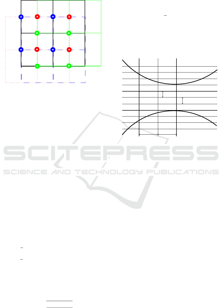
p
i+1,j
, T
i+1,j
p
i+1,j+1
, T
i+1,j+1
p
i,j
, T
i,j p
i,j+1
, T
i,j+1
u
i+1,j−1/2
u
i,j−1/2
u
i+1,j+1/2
u
i,j+1/2
v
i−1/2,j
v
i−1/2,j+1
v
i+1/2,j
v
i+1/2,j+1
Figure 1: Staggered grid with the calculation nodes.
where n
1
,n
2
∈ R denotes the number of discretisa-
tion lines in x and y direction, respectively and i =
1,2,...,n
1
and j = 1,2,...,n
2
are the indices of the
cells. f represents any of considered variables on cer-
tain node of the grid, which will be treated through the
corresponding operator listed above and ∆x is the dis-
cretisation step in x direction. In y-direction we de-
fine the operators D
y
,D
y
−
,D
y
+
and K
y
similarly. With
these operators we can discrete our PDAE-system (1)
- (4) and we get the equations
I
˙
u(t) = K(u)u(t) − Bp(t)+ f (u(t), p(t)) (9)
0 = B
T
u(t) (10)
I
˙
T (t) = K
1
(u)T (t)+ D(u) + g(T (t)), (11)
where I is the identity matrix, B = [D
x
+
,D
y
+
]
T
is the
discrete divergence operator and K(u) = (K + N(u)),
with K = [K
x
,K
y
]
T
representing the linear (difusion)
and
N(u) =
"
u
i, j+1/2
D
x
+ v
∗
i, j+1/2
D
y
u
∗
i+1/2, j
D
x
+ v
i+1/2, j
D
y
#
representing the nonlinear (convection) terms. The
velocity u
∗
i+1/2, j
and v
∗
i, j+1/2
are average velocities de-
fined by the four velocities around the point v
i+1/2, j
or
u
i, j+1/2
:
u
∗
i+1/2, j
=
1
4

u
i, j−1/2
+ u
i, j+1/2
+ u
i+1, j+1/2
+ u
i+1, j−1/2

v
∗
i, j+1/2
=
1
4

v
i−1/2, j
+ v
i+1/2, j
+ v
i+1/2, j+1
+ v
i−1/2, j+1

The forcing functions f(u(t), p(t)) and g(T (t)) in
the equations (9) and (11) comes from the boundary
conditions. The operator K
1
(u) = (K + N
1
(u)) for
the temperature calculation has the convection term
N
1
(u) this can by described by:
N
1
(u) =
"
u
i, j−1/2
+u
i, j+1/2
2
D
x
v
i−1/2, j
+v
i+1/2, j
2
D
y
#
The Term D(u) is defined by
D(u) = 2η((D
x
+
u)
2
+
1
η
(D
y
+
u + D
x
+
v)
2
+ (D
y
+
v)
2
).
With these presented discrete operators we receive the
equations (9) - (11).
In Fig. 2 it is to be taken that the use of a rectan-
gular grid causes individual grid points to be located
outside the fluid area.
∆y
∆x
∆y
∆x
Figure 2: Rectangular equidistant grid.
With this background, a curvilinear grid is used in
this case, where the step size ∆x is constant, while ∆y
is varied along the flow direction, see Fig. 3. Ana-
logous to the rectangular grid, the calculation points
for the velocities are located at the center of the cell
edge and the points for pressure and temperature at
the center of the cell. Comparing both different grids
and assuming a constant number of cells at the narro-
west gap, e.g. four cells (as in Fig. 2 and 3. represen-
ted), results a higher dimensioned DAE-System from
rectangular grid than using curvilinear grid. For ex-
ample in our case we get for the identity matrix for the
rectangluar grid I
rec
∈ R
78×50
and for the curvilinear
grid I
cur
∈ R
5×50
. The main advantage of a curvilinear
grid is therefore a lower calculation effort. However,
a sensible use of the curvilinear grid is only possible
with sufficiently large radii, since there is the risk of
an inaccurate calculation with small radii.
4 SOLUTION PROCEDURE
In order to solve the Navier-Stokes equations (9) -
(10) on the basis of the Finite-Difference-Method
(FDM), a pressure correction method, the projection
method based on Chorin (Chorin, 1968) is used. The
projection method is as follows (Weickert, 1996)
Modelling and Simulation of High-viscosity, Non Iso-thermal Fluids with a Free Surface
559

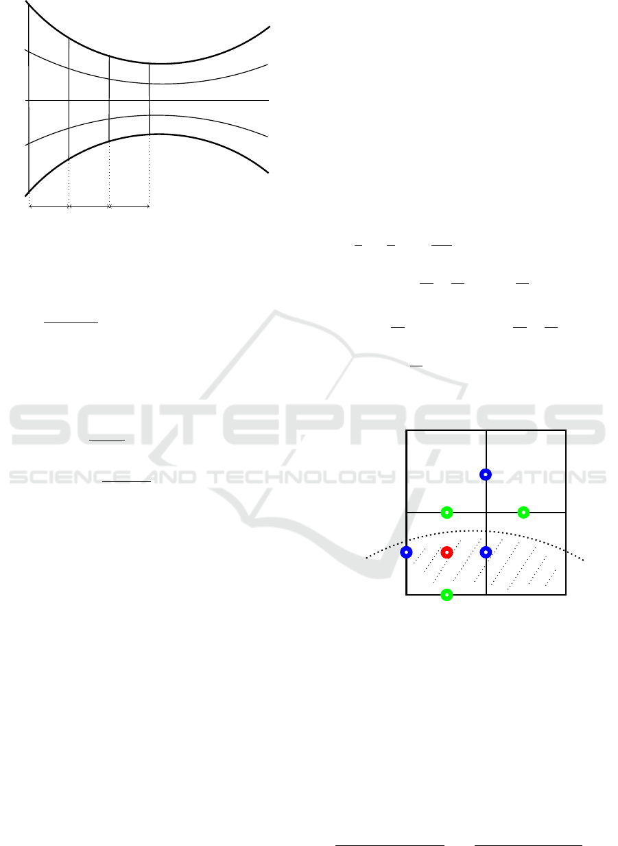
∆y
i
∆y
i
∆y
i
∆y
i
∆y
i+1
∆y
i+1
∆y
i+1
∆y
i+2
∆y
i+2
∆y
i+2
∆y
i+3
∆y
i+3
∆y
i+3
∆y
i+3
∆x∆x∆x
∆y
i+2
∆y
i+1
Figure 3: Curvilinear grid.
• Perform a semi-implicit time discretiziation with
∆t as time discretization parameter and n + 1 as
the number of the current time step:
u
n+1
− u
n
∆t
= K(u
n
)u
n
− Bp
n+1
+ f
n+1
(12)
0 = B
T
u
n+1
(13)
• Decouple the pressure from the momentum equa-
tion (12) and calculate the pseudo velocities
˜
u
from the equation (14)
˜
u − u
n
∆t
= K(u
n
)u
n
+ f
n+1
(14)
u
n+1
−
˜
u
∆t
= −Bp
n+1
(15)
• Applying the dicrete divergence operator B on
(15) we obtain the Poisson equation (16) and the
equation for u
n+1
∆tB
T
Bp
n+1
= B
T
˜
u (16)
u
n+1
=
˜
u − ∆tBp
n+1
(17)
This strategy can be described by the strangeness free
DAE-system (Weickert, 1996)

I 0
0 0

˙
u
˙p

=

K(u) 0
−B
T
∆tB
T
B

u
p

+

f
0

.
The temperature is calculated from (11) with the cor-
rected speed values. The free surface is then determi-
ned.
5 DETERMINATION OF THE
FREE SURFACE
The MAC method used here is found in the essays
(Amsden and Harlow, 1970; Tome and McKee, 1994)
and is used for determining the free surface. Massless
particles are used to mark those cells that are partially
or completely filled by the fluid. In other words, each
cell in which includes at least one massless particle is
part of the area in which the fluid is located. Against
this background, the massless particles are also called
markers. If there are empty cells border on a fluid cell,
then this fluid cell is the one where the free surface
passes. Such constellations are shown in Fig. 4 and
5. On a free surface for incompressible fluids, nor-
mal and tangential stresses are equal to zero, cf. (Hirt
and Shannon, 1968; Nichols and Hirt, 1971). For a
two-dimensional surface, the two following conditi-
ons apply
p
ρ
− 2
η
ρ

n
x
n
x
∂u
∂dx
+ n
x
n
y

∂u
∂y
+
∂v
∂x

+ n
y
n
y
∂v
∂y

= 0,
(18)

2n
x
m
x
∂u
∂x
+ (n
x
m
y
+ n
y
m
x
)

∂u
∂y
+
∂v
∂x

+2n
y
m
y
∂v
∂y

= 0,
(19)
where n = (n
x
,n
y
) is the outward-looking normal and
m = (m
x
,m
y
) = (n
y
,−n
x
) is the tangential vector.
p
i,j
u
i,j−1/2
u
i,j+1/2
u
i+1,j+1/2
v
i−1/2,j
v
i+1/2,j
v
i+1/2,j+1
Figure 4: Marked cell with a free adjacent cell.
The free surface conditions are determined by the
adjacent free cells, which is explained below using
two examples. In Fig. 4 the lower left cell has one
side bordering on a free cell. In this example, the nor-
mal component n
x
is very small and (18) and (19) can
be discretized and simplified to
p
i, j
− 2η

D
y
+
v

= 0, (20)
and
D
y
+
u = −D
x
+
v
u
i+1, j+1/2
− u
i, j+1/2
∆y
i, j+1/2
= −
v
i+1/2, j+1
− v
i+1/2, j
∆x
(21)
ICINCO 2018 - 15th International Conference on Informatics in Control, Automation and Robotics
560

p
i,j
u
i,j−1/2
u
i+1,j+1/2
v
i−1/2,j
v
i+1/2,j
Figure 5: Marked cell with two free adjacent cells.
The pressure p
i, j
for the cell in Fig. 4 is calculated
from (20) and the speed u
i+1, j+1/2
is calculated from
(21), whereby the free surface conditions are fulfilled.
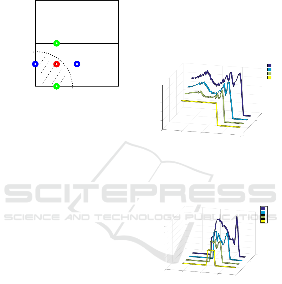
Other scenarios, in which the selected cell borders on
only one side of an empty cell, are simplified in the
same way. In Fig. 5 two empty cells adjacent on the
fluid cell, in such a scenario it is assumed that the
normal vector points at an angle of 45
◦
to the open
sides. In this case (18) and (19) are simplified to
p − η

D
y
+
u + D
x
+
v

= 0 (22)
and
D
x
+
u − D
y
+
v = 0.
(23)
In Fig. 5 the pressure is calculated based on (22) and
the speeds u
i+1, j+1/2
and v
i+1/2, j
are equal to the op-
posite speeds of the fluid cell, so that (23) is fulfilled.
Further scenarios, which can occur, can be found e.
g. in (Amsden and Harlow, 1970; Tome and McKee,
1994).
6 RESULTS
Although the numerical results include the local and
temporal course of the velocities, pressures and tem-
peratures of the fluid, only individual temperature
profiles of the fluid along the flow direction of three
different layers at four different points in time are
shown below. The temperature at time t
1
, in all fi-
gures corresponds to the initialized area of fluid. The
initialized temperature of the fluid is 425 Kelvin and
the ambient temperature is 400 Kelvin. In Fig. 6 the
fluid is attached to a cylinder with a constant tempe-
rature of 435 Kelvin. As the fluid moves forward as a
result of cylinder rotation, the fluid is entering the gap.
The change of pressure gradient due to the narrowing
of the space between the cylinders, couses the acce-
leration respectiveley the deceleration of the different
fluid layers. This leads to shearing of the fluid thus in
an increase of temperature, so that the fluid partially
assumes temperatures higher than the cylinder tempe-
rature. From the point where the shear decreases, the
cylinder thus contributes to the cooling of the hotter
fluid. The temperature profile at time t
4
shows in Fig.
6 also a shift to the right. This indicates that the fluid
has flowed through the gap between the cylinders.
0
2
t
n
Temperature Profiles
4
400
-0.15
410
x [m]
-0.1
420
-0.05
T [K]
6
0
430
0.05
440
450
t
4
t
3
t
2
t
1
Figure 6: Temperature profiles of the layer adjacent to the
upper cylinder.
The change in the temperature profile of the
middle and the layer adjacent to the lower cylinder,
see Fig. 7 and 8, is based on the same physical pro-
cesses (shear, etc.) that have caused the temperature
change of the layer adjacent to the upper cylinder.
0
2
t
n
Temperature Profiles
4
400
410
-0.15
x [m]
420
-0.1
430
-0.05
T [K]
6
440
0
450
0.05
460
470
t
4
t
3
t
2
t
1
Figure 7: Temperature profiles of the middle layer.
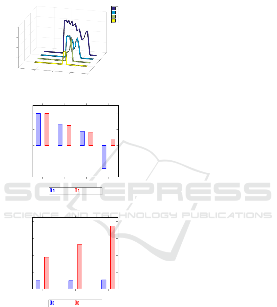
In the Fig. 8 you can also see that the fluid in in-
dividual areas not only moves in the direction of the
cylinder gap but also accumulates in individual pla-
ces.
In Fig. 9 it can be seen that with a decreasing cy-
linder radius from one point upwards there is a signi-
ficant deviation in the resolution of the velocity com-
pared to the rectangular grid. This is partly due to the
fact that small radii lead to increased curvature radii
and thus in some places there are too large step widths
in the y-direction and this causes numerical errors.
Fig. 10 shows the normalized calculation time be-
tween the grids required for 100000 time steps. As
Modelling and Simulation of High-viscosity, Non Iso-thermal Fluids with a Free Surface
561

0
2
t
n
Temperature Profiles
4
400
-0.15
420
x [m]
-0.1
-0.05
440
6
T [K]
0
0.05
460
480
t
4
t
3
t
2
t
1
Figure 8: Temperature profiles of the layer adjacent to the
lower cylinder.
r=40 cm r=29 cm r=21 cm r=17 cm
−0.5
0
0.5
1
1
0.66
0.44
−0.73
1
0.63
0.41
0.2
normalized speed
curvilinear rectangular
Figure 9: Normalized speed at a point with constant rpm
and variable radius of the cylinders.
5 8 12
2
4
6
8
1
1.02
1.1
3.77
5.3
7.5
normalized time
curvilinear rectangular
Figure 10: Normalized calculation time of 100000 time
steps with 5,8 and 12 calculation nodes at the narrowest gap.
already mentioned before, the high calculation time
for the rectangular grid results from the higher num-
ber of calculation nodes. In the comparison, the num-
ber of calculation nodes in the y-direction for both
calculation grids was kept constant at the narrowest
gap. Casewise, resulting dimensions for curvilinear
grid are 5x50, 8x50 and 12x50, respectiviley 78x50,
136x50 and 215x50 for the rectangular grid. It should
be mentioned that the computional time step in both
grids is the same. Thus the calculation time is only
dependent on the dimension of the grid and not on the
time step size as in (Morianou et al., 2016), where the
time step size in the rectangular grid is smaller than
in the curvilinear grid.
7 CONCLUSIONS
This paper presents a mathematical model of a non-
isothermal, high-viscosity fluid that flows between
two counter-rotating cylinders. In combination with
the MAC method, the model offers the possibility to
determine the course of the free surface. For this pur-
pose, the underlying distribution parametric model is
discretized with respect to numerical simulation on
a curvilinear grid and not, as usual, on a rectangular
grid. Since with a curvilinear grid, the edge of the cy-
linders is identical to the outer lines of the discretizing
grid, the system of differential-algebraic equations re-
sulting from the spatial discretization is reduced com-
pared to that of a rectangular grid. However, a sen-
sible use of the curvilinear grid is only possible with
sufficiently large radii. Due to the coarser discretiza-
tion, too small radii typically lead to inaccurate calcu-
lation results. The aspect of how an increased radius
of curvature exactly affects a numerical error is to be
further analysed and the comparison of the quality of
both models to measured data on a real system is to
take place in more advanced work.
REFERENCES
Aamo, O. M. and Krstic, M. (2003). Flow Control by Feed-
back: Stabilization and Mixing. Springer.
Amsden, A. A. and Harlow, F. H. (1970). The smac method:
A numerical technique for calculation incompressible
fluid flows. Technical report, Los Alamos Scientific
Laboratory of the University of California.
Chorin, A. J. (1968). Numerical solution of the navier-
stokes equations. Mathematics of Computation,
22(104):745–762.
Dellar, O. J. and Jones, B. L. (2016). Discretising the line-
arised navier-stokes equations: A systems theory ap-
proach. UKACC International Conference on Control
(Control).
Harlow, F. H. and Welch, J. E. (1965). Numerical calcu-
lation of time-dependent viscous incompressible-flow
of fluid with free surface. The Physics of Fluids,
8(12):2182 – 2189.
Hirt, C. W. and Shannon, J. P. (1968). Free-surface stress
conditions for incompressible-flow calculations. Jour-
nal of Computational Physics, 2:403 – 411.
ICINCO 2018 - 15th International Conference on Informatics in Control, Automation and Robotics
562

Hou, T. Y. and Wetton, B. T. R. (1993). Second-order con-
vergence of a projection scheme for the incompressi-
ble navier-stokes equations with boundaries. Society
for Industrial and Applied Mathematics.
Jones, B. L., Heins, P. H., Kerrigan, E. C., Morrison, J. F.,
and Sharma, A. (2015). Modelling for robust feedback
control of fluid flows. Journal of Fluid Mechanics,
769:687–722.
Jovanovic, M. and Bamieh, B. (2001). Modeling flow statis-
tics using the linearized navier-stokes equations. Con-
ference on Decision and Control.
McKee, S., Tome, M., Ferreira, V., Cuminato, J., Castelo,
A., Sousa, F., and Mangiavacchi, N. (2008). The mac
method. Computer & Fluids.
Morianou, G. G., Kourgialas, N. N., and Karatzas, G. P.
(2016). Comparison between curvilinear and rectili-
near grid based hydraulic models for river flow simu-
lation. Procedia Engineering, 162:568 – 575.
Nichols, B. D. and Hirt, C. W. (1971). Impro-
ved free surface boundary conditions for numerical
incompressible-flow calculations. Journal of Compu-
tational Physics, 8:434–448.
Tome, M., Filho, A., Cuminato, J., Mangiavacchi, N., and
McKee, S. (2000). Gensmac3d: a numerical method
for solving unsteady three-dimensional free surface
flows. International Journal for Numerical Methods
in Fluids.
Tome, M. F. and McKee, S. (1994). Gensmac: A computa-
tional marker and cell method for free surface flows in
general domains. Journal of Computational Physics,
110:171–186.
Weickert, J. (1996). Navier-stokes equations as a
differential-algebraic system. Technical report,
Technische Universitt Chemnitz-Zwickau.
Weston, B. (2000). A marker and cell solution of the in-
compressible navier-stokes equations for free surface
flow. Technical report, Department of Mathematics
University of Reading.
Modelling and Simulation of High-viscosity, Non Iso-thermal Fluids with a Free Surface
563