A Multi-source Machine Learning Approach to Predict Defect Prone

Components

Pasquale Ardimento

, Mario Luca Bernardi

and Marta Cimitile

Computer Science Department, University of Bari Aldo Moro, Via E. Orabona 4, Bari, Italy

Department of Computing, Giustino Fortunato University, Benevento, Italy

Unitelma Sapienza, Rome, Italy

Keywords:

Machine Learning, Fault Prediction, Software Metrics.

Abstract:

Software code life cycle is characterized by continuous changes requiring a great effort to perform the testing

of all the components involved in the changes. Given the limited number of resources, the identiﬁcation of

the defect proneness of the software components becomes a critical issue allowing to improve the resources

allocation and distributions. In the last years several approaches to evaluating the defect proneness of software

components are proposed: these approaches exploit products metrics (like the Chidamber and Kemerer metrics

suite) or process metrics (measuring speciﬁc aspect of the development process). In this paper, a multi-

source machine learning approach based on a selection of both products and process metrics to predict defect

proneness is proposed. With respect to the existing approaches, the proposed classiﬁer allows predicting the

defect proneness basing on the evolution of these features across the project development. The approach is

tested on a real dataset composed of two well-known open source software systems on a total of 183 releases.

The obtained results show that the proposed features have effective defect proneness prediction ability.

1 INTRODUCTION

Add new features and/or increase the software qua-

lity require much effort invested to perform software

testing and debugging. However, software developers

resources are often limited and the schedules are very

tight. Defect prediction can support developers and

reduce the resources consumption through the iden-

tiﬁcation of the software components that are more

prone to be defective. Basing on the above consi-

derations, several defect prediction machine learning

classiﬁcation approaches (Radjenovi

c et al., 2013) are

proposed in the last years. They are based on a clas-

siﬁer that predicts defect-prone software components

basing on a set of features (i.e, code complexity, num-

ber of code lines, number or modiﬁed ﬁles) (Isong

et al., 2016). Basing on the more recent studies (Rad-

jenovi

c et al., 2013), several machine learning ba-

sed approaches adopt product metrics like Chidamber

and Kemerer’s (CK) (Chidamber and Kemerer, 1994;

Boucher and Badri, 2016) object-oriented metrics as

features. Even if these products metrics are surely

highly correlated to defects as several studies con-

ﬁrms (Hassan, 2009), there are also other aspects, re-

lated to the adopted development process, that need to

be taken into account to capture the complex techni-

cal and social implications of the phenomenon of bug

introduction in a predictive model. In this paper a new

machine learning approach to predict defect prone

components is proposed. Differently, from the other

approaches, the proposed classiﬁer uses as features

the evolution over releases of a mix of products and

process metrics.

Section 2 discusses the related work and the back-

grounds. Section 3 introduces the proposed classiﬁca-

tion process while Section 4 presents the evaluation of

the proposed features effectiveness referring to their

capability to evaluate the software code proneness and

discusses the results of the evaluation. Finally, paper

conclusions and future work are reported in Section

2 RELATED WORK

The defect prediction approaches proposed in litera-

ture apply data mining and machine learning algo-

rithms to classify the software components into de-

fective or non-defective. These approaches utilize

272

Ardimento, P., Bernardi, M. and Cimitile, M.

A Multi-source Machine Learning Approach to Predict Defect Prone Components.

DOI: 10.5220/0006857802720279

In Proceedings of the 13th International Conference on Software Technologies (ICSOFT 2018), pages 272-279

ISBN: 978-989-758-320-9

a classiﬁcation model obtained from the analysis of

the earlier projects data considered as features (Les-

smann et al., 2008). According to the literature (Bou-

cher and Badri, 2016), several approaches are ba-

sed on the adoption of CK metrics suite introduced

in (Chidamber and Kemerer, 1994). Two experi-

ments on the relation between object-oriented design

metrics and software quality are proposed in (Basili

et al., 1996; Briand et al., 2000). In (Kanmani et al.,

2007), the effectiveness of the CK metrics for soft-

ware fault prediction is evaluated by using two neu-

ral network based models. Similarly, multiple linear

regression, multivariate logistic regression, decision

trees and Bayesian belief network are used respecti-

vely in (Nagappan et al., 2005; Olague et al., 2007;

Gyimothy et al., 2005; Kapila and Singh, 2013). In

(Lessmann et al., 2008) a framework for comparative

software prediction is proposed and tested on 22 clas-

siﬁers and 10 NASA datasets. The obtained results

show an encouraging predictive accuracy of the clas-

siﬁers and no signiﬁcant difference in the classiﬁers

performances. Finally, in (Kaur and Kaur, 2018), the

six better (basing on the previous studies) classiﬁca-

tion algorithms are used to compare models for fault

prediction on open source software and compare the

results of open software projects with an industrial da-

taset. The analysis of the literature shows that most

studies on software defect prediction are focused on

a comparative analysis of the available machine lear-

ning methods. In this paper, we propose a features

model that takes into consideration the software com-

ponent’s history to consider the evolution of a mix

of products and process metrics. The novelty resides

in the application of an ensemble learning approach

using the selected set of products and process metrics

evaluated at different observation points in space (i.e.

the project’s classes) and time (i.e. at each release).

This allows training a classiﬁer that becomes more ef-

fective as the software project matures (i.e. more re-

leases are generated) since more training data is avai-

lable.

3 THE METHODOLOGY

The key aspects of our approach are the granularity of

prediction (i.e. the code elements selected as the tar-

gets of the prediction), the metrics exploited as featu-

res, the adopted machine learning prediction techni-

ques.

For that concerns the granularity, the proposed ap-

proach aims at identifying the defects at a class le-

vel. This means evaluating the defect proneness of a

class across software project releases events. Most of

the existing defect proneness prediction approaches

are able to predict the defects only at source ﬁle level

(Hassan, 2009; Moser et al., 2008) or, even worse, at

the component level (Nagappan et al., 2010). Coarse-

grained predictions force developers to spend effort in

locating the defects. Since ﬁner granularity, instead,

can mitigate such issue, the proposed model has been

designed to predict the defects at class level thus ef-

fectively restricting the testing effort required.

For what concerns features selection, there are

two classes of metrics that are widely used to predict

bugs: product metrics, that characterize features of

the source code elements; process metrics, that cha-

racterize the development history of the source code

elements. To take into account all these aspects when

predicting defects, the proposed approach exploits a

mix of the ﬁrst two classes of features.

The last key aspect is the prediction technique ex-

ploited in our approach. In literature, machine lear-

ning techniques have been successfully exploited for

bug prediction. These approaches(Moser et al., 2008),

mostly adopting supervised learning, seems to sug-

gest that the impact of the adopted metrics on the clas-

siﬁcation performances is much higher than the speci-

ﬁc machine learning algorithm chosen to perform the

classiﬁcation. To conﬁrm this, in our study several

classiﬁcation techniques based on supervised learning

are compared and results discussed.

The overall defect proneness classiﬁcation process

is summarised in Figure 1 and the remaining of the

section delves into the details of each step.

3.1 Data Collection

The process starts with the data collection step repre-

sented in Figure 1-(a) that extracts the information

from the source code repository and the bug tracking

system and integrates them into a single coherent da-

taset. The required information is spread between the

issue tracker (BTS) and the source code repository

(VCS). Such integration is centered on recovering the

traceability links among the two systems to identify

the commits making up each release and linking the

issues reported in BTS to them.

To this regards a tool, written in Java, has been

developed to execute the following tasks, for a given

software project: downloads the VCS repository; eva-

luates the total number of releases, commits and the

total number of commits for each release; calculates,

for each release, all the revisions (commit IDs) that

are related to it; collects information about commit

date, commit author, commit URL, and other struc-

tural information. Then two scripts have been deve-

loped to automate the extraction process. The ﬁrst

A Multi-source Machine Learning Approach to Predict Defect Prone Components

273

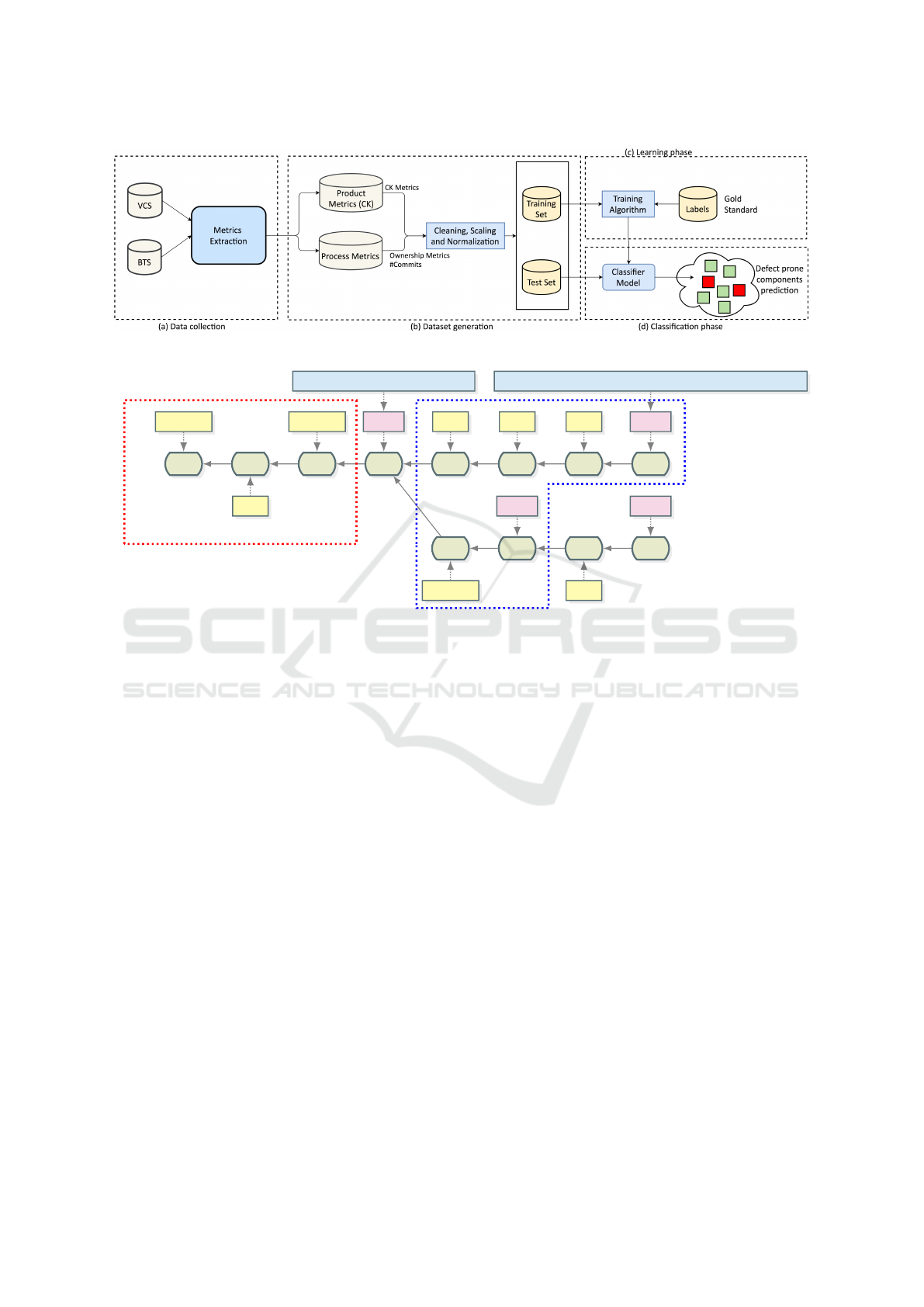
Figure 1: An overview of the defect prone components prediction process.

123b f7ab 4e1c 8d1c eb10 f2c2 5b0b 8c86

ffc6 0b3b 1ab7 5ca2

Fix 5Feature 3

Fix 4Fix 2

v1.1.1

Fix 3 v1.0.1

v1.1.0

v1.0.0

Fix 1

Feature 2Feature 1

Metrics on commits 123b,f7ab,4ec1 Metrics on commits 123b,f7ab,4ec1,8d1c,eb10,f2c2,5b0b,8c86

Commits for metrics evaluation of release v1.0.0

Commits used to generate labels for release v1.0.0

Figure 2: A small excerpt of a typical repository graphs, decorated with information on Issues, Bugs and Fixes.

script builds automatically all the release source co-

des, using Apache Ant or Apache Maven, while the

second one evaluates the metrics of different classes

and stores the results. A broad overview of the in-

tegration is depicted on Figure 2. A key problem in

evaluating the metrics is to deﬁne the portion of the

source code repository graph that is used for each re-

lease. Our approach, given the commit of a release

(e.g. commit ID 8d1c in the ﬁgure), creates a set of

commits that, for that release, is built by following

back the parent/children relationship of the repository

DAG until to the branch root (this set is highlighted

in red in Figure 2). For each commit found on this

path, information gathered from BTS are considered

in order to evaluate required metrics. Speciﬁcally, as

Figure 1 shows, from these integrated data sources,

two classes of defect predictors (product and process

metrics) are generated and are used, later in the pro-

cess, as features for the subsequent learning step.

3.1.1 Product Metrics

We selected a subset of the Chidamber-Kemerer (CK)

ObjectOriented (OO) Metric Suite(Chidamber and

Kemerer, 1994), reported in Table 1. To evaluate

these metrics, the CKJM tool developed by Spinel-

lis(Spinellis, 2005) was integrated into our toolchain

to perform the experimentation. This tool is able

to calculate Chidamber and Kemerer object-oriented

metrics for each class of the system, by processing the

bytecodes of compiled Java ﬁles. This means that, for

each release, a complete snapshot of the entire source

code must be extracted and compiled to produce the

bytecodes feeding the CKJM tool.

3.1.2 Process Metrics

Since there are several factors, related to the deve-

lopment process with which the software project is

developed, inﬂuencing the complex phenomenon of

bug introduction. For this reason, process metrics

are also taken into account looking at both the kind

of changes that are performed and the properties of

committers performing such changes. Table 2 reports

the process metrics considered as features. To evalu-

ate the number of commits, issues, and bugs for each

class we build the log from the VCS repository and

extract, for each commit, the ﬁles changed, the com-

mit ID, the commit timestamp, the committer ID, and

the commit note. With this information, we are also

ICSOFT 2018 - 13th International Conference on Software Technologies

274

Table 1: Product Metrics adopted as features to train the

classiﬁer.

Metric Description

WMC

Weighted Method per Class - It mea-

sures the complexity of a class calcu-

lated by the cyclomatic complexities of

its methods

DIT

Depth of Inheritance Tree - It calculates

how far down a class is declared in the

inheritance hierarchy.

NOC

Number of Children - It calculates how

many sub-classes are going to inherit

the methods of the parent class.

CBO

Coupling Between Objects - It evalua-

tes the coupling between objects.

RFC

Response for a Class - The number of

methods that can be invoked in response

to a message in a class.

LCOM

Lack of Cohesion in Methods - It me-

asures the amount of cohesiveness pre-

sent.

Afferent Couplings - It evaluates the

number of classes that depend upon the

measured class

NPM

Number of Public Methods - It evalu-

ates all the methods in a class that are

declared as public

Table 2: Process Metrics adopted as features to train the

classiﬁer.

Metric Description

#Commits

The number of total commits on the

class.

#Issues

The number of total issues (Impro-

vements, Refactoring, and Tasks) in-

volving the class.

#Bugs

The number of total bugs involving

the class.

#Owner

Commit-

ters

The number of owners that have

worked on the class.

#Other

Commit-

ters

The number of other committers (i.e.

committers not owning the class)

that have worked on the class.

#Commits

by Others

The number of total commits on the

class performed by committers not

owning the class.

able to identify ﬁx-inducing changes using an appro-

ach inspired by the work of Fischer (Fischer et al.,

2003), i.e., we select changes with the commit note

matching a pattern such as bug ID, issue ID, or si-

milar, where ID is a registered issue in the BTS of

the project. Hence the issue ID acts as traceability

link between VCS and BTS systems. We then use

the issue type/severity ﬁeld to classify the issue and

distinguish bug ﬁxing changes from different kind of

issues (e.g., improvement, enhancements, feature ad-

ditions, and refactoring tasks). This is needed to com-

pute, for each class, the process metrics (the number

of improvement/refactoring issues and the number of

ﬁxes). Finally, we only consider issues having the

status CLOSED and the resolution FIXED since their

changes must be committed in the repository and ap-

plied to the components in the context of a release.

Basically, we distinguish among: (i) issues that were

related to bugs, since we use them as a measure of

fault-proneness, and (ii) issues that are related to im-

provement and changes.

To identify ﬁx-inducing changes, we use a modi-

ﬁed version of SZZ algorithm presented in (Kim et al.,

2008). It is based on the git blame feature which, for

a ﬁle revision, provides for each line the revision of

the last change occurred in time. More precisely, gi-

ven the ﬁx for the bug identiﬁed by k, the approach

proceeds as follows:

1. let p(c) be the parent of the commit c; for each

ﬁle f

, i = 1 . . . m

involved in the bug ﬁx k (m

the number of ﬁles changed in the bug ﬁx k) and

ﬁxed in a commit with ID R

f ix

i,k

, we get the same

ﬁle in its parent commit with ID p(R

f ix

i,k

), since

it is the most recent revision that still contains the

bug k.

2. starting from the revision with commit ID

p(R

f ix

i,k

), the blame command of git is used to

detect, for each line in f

changed in the ﬁx of

the bug k, the commit, in the past, where the last

change to that line occurred. Hence for each ﬁle

, we obtain a set of n

i,k

ﬁx-inducing commit IDs

i, j,k

, j = 1 . . . n

i,k

The revisions R

i, j,k

, j = 1 . . . n

i,k

are ﬁnally used to

perform bugs and issues counting aggregating by ﬁle

and by release in order to evaluate the a subset of pro-

cess metrics (i.e. the number of commits, ﬁxes and

bugs for each class in each release).

However further information is required to evalu-

ate metrics related to ownership (i.e. the number of

owners committers, the number of other committers

and the number of commits on each class performed

by the other committers).

In (Bird et al., 2011) authors deﬁned a ﬁle owner

as a committer that performed, on a ﬁle, a given per-

centage of the total number of commits occurred on

that ﬁle. Hence we tag as owners the set of the com-

mitters of a ﬁle that collectively performed at least

half of the total commits on that ﬁle.

More formally, we identify as the set of ﬁle ow-

A Multi-source Machine Learning Approach to Predict Defect Prone Components

275

ners for ﬁle f

at time t the set:

O( f

, t) ≡ {o

, . . . , o

} (1)

of committers that, overall, performed the 50% of

commits on f

in the time interval [0, t] (where 0 is

the starting point of our period of observation), i.e.,

|O( f

,t)|

∑

j=1

C(o

) ≥ 0.5 · T

( f

, t) (2)

where C(o

) is the number of commits performed by

on ﬁle f

in the time interval [0, t], and T

( f

, t) is

the total number of commits performed on f

in the

time interval [0, t]. To calculate the set O( f

, t), we

build an ascending sorted list of committers based on

the number of commits they performed on f

in the

time interval [0, t], and selected the minimum set of

topmost committers in the ranked list that satisﬁes the

above constraint.

By collecting all these metrics for each class of the

system, at a given release, the feature vector reported

in Figure 3 is constructed and used for training.

3.2 Dataset Generation Steps

The goal of this step, reported in Figure 1-(b), is to

produce a dataset from the metrics evaluated from

data sources that are suitable to be used to train a clas-

siﬁer adopting a supervised machine learning appro-

ach. The labeled match data consists of all the com-

mits performed on the ﬁxed ﬁle and the corresponding

values of the metrics. The labeled match data is ﬁrstly

cleaned (by removing the incomplete and wrong data)

and normalized.

The cleaning consists of polish data produced du-

ring the pre-processing step in order to: i) ﬁx missing

values; ii) remove noise; iii) remove special character

or values; iv) verify semantic consistency.

After the cleaning, the normalization is performed

by using a Min-max scaling approach realizing a li-

near transformation of the original data. More preci-

sely, if min

is the minimum value for the attribute X

and max

is the maximum for X, the min-max nor-

malization approach relates a value v

of X to a v

the range {newMin

, newMax

} by computing:

− min

max

− min

(newMax

−newMin

)+newMin

From the normalized data, a dataset is derived. It

contains the training set used to train the classiﬁer and

the test set used to make the performance assessment

of the classiﬁer.

3.3 Learning Phase

To perform the learning phase is necessary to calcu-

late the labels (i.e. the defective components of relea-

ses used for training the classiﬁer). Given a release X,

we construct such labels by looking at the future com-

mits until we reach on each subsequent branch the

next releases. This allows considering ﬁxes that apply

to release X and from them recover, as already discus-

sed, the ﬁx-inducing changes. Files affected by ﬁx-

inducing changes are ﬁnally labeled as DEFECTIVE

or NOT-DEFECTIVE.

The training is performed using a stratiﬁed K-fold

cross-validation (Rodriguez et al., 2010) approach. It

consists to split the data into k folds of the same size in

which the folds are selected so that each fold contains

roughly the same proportions of class labels. Subse-

quently, k iterations of training and validation are per-

formed and, for each iteration, a different fold of the

data is used for validation while the remaining folds

are used for training. As pointed out, to ensure that

each fold is representative, the data are stratiﬁed prior

to being split into folds. This model selection method

provides a less biased estimation of the accuracy.

3.4 Classiﬁcation Phase

In this step, the trained classiﬁer is ready to be used

to perform prediction on new data extracted from the

project. It could be applied to the live software project

data and can be used to predict, at the current release,

what are the classes that are the most likely to produce

bugs until the next release cycle. Since the approach

works on metrics that can be automatically extracted,

it is suitable to be integrated into existing BTS or con-

tinuous integration (CI) platforms.

4 EVALUATION

4.1 Experiments Description

To validate the approach, an experiment was perfor-

med involving the following two projects, both writ-

ten in Java Language: Apache CXF, a well known

open source services framework, and Apache Com-

mons IO, a widespread library that contains several

facilities for text and binary data management. The

dataset for Apache CXF contains 134 releases (from

release 2.1 up to release 3.2.0), while the dataset for

Apache Commons IO contains 49 releases (from re-

lease 1.0.0 up to release 2.5.0).

The experimentation was performed by using the

classiﬁers, reported in Table 3, based on traditional

ICSOFT 2018 - 13th International Conference on Software Technologies

276

Figure 3: The features vector used to train the classiﬁer.

Table 3: Machine-learning classiﬁcation algorithms.

Classiﬁcation

Alghoritm

Description

J48

A decision tree is created based on the attribute values of the training dataset in order to

classify a new item. The set of items discriminating the various instances is extracted so

when a new item is encountered it can be classiﬁed.

Decision

Stump

It consists to create a decision tree model with one internal root node immediately con-

nected to the terminal nodes. The prediction is allowed by a decision stump basing on the

value of just one input feature.

Hoeffding

Tree

An incremental, anytime DT induction algorithm learning from massive data streams.

Basing on the assumption that the distribution generating examples does not change over

time, it often uses a small sample to choose an optimal splitting attribute.

Random

Forest

It operates by constructing, at training time, a multitude of DTs and outputting the class

that is the mode (the most frequent value appearing in a set of data) of the classes of the

individual trees.

Random Tree

It constructs a tree containing some randomly chosen attributes at each node. No pruning

is performed.

REP Tree

It builds a DT using information gain/variance and reduces errors using reduced-error pru-

ning. The values are ordered for numeric attributes once and missing values are recovered

with by splitting the corresponding instances into pieces.

Table 4: Best Precision, Recall and F-Measure for Apache

CXF for the adopted learning algorithms.

Algorithm P R F Class

0.82 0.88 Defective

J48 0.83 0.89 0.85 Not defective

0.79 0.78 Defective

Decision

Stump

0.81 0.71 0.78 Not defective

0.86 0.89 Defective

Hoeffding

Tree

0.88 0.91 0.89 Not defective

0.87 0.88 Defective

Random

Forest

0.87 0.90 0.87 Not defective

0.85 0.81 Defective

Random

Tree

0.83 0.86 0.83 Not defective

0.80 0.81 Defective

REPTree 0.77 0.72 0.80 Not defective

Machine Learning (ML) algorithms: J48, Decision-

Stump, HoeffdingTree, RandomForest, RandomTree

and REPTree. A description of these algorithms is

also reported in the same table. They all use a de-

cision tree as a predictive model. The observations

about an item are represented as the branches of the

tree and they are used to obtain conclusions about its

class (the leaves of the tree).

Table 5: Best Precision, Recall and F-Measure for Apache

Commons-IO for the adopted learning algorithms.

Algorithm P R F Class

0.71 0.77 Defective

J48 0.74 0.80 0.70 Not defective

0.68 0.69 Defective

Decision

Stump

0.70 0.60 0.66 Not defective

0.78 0.81 Defective

Hoeffding

Tree

0.80 0.83 0.82 Not defective

0.76 0.77 Defective

Random

Forest

0.75 0.81 0.78 Not defective

0.74 0.72 Defective

Random

Tree

0.76 0.75 0.74 Not defective

0.71 0.72 Defective

REPTree 0.66 0.64 0.68 Not defective

4.2 Evaluation Strategy

To validate the classiﬁer we used the following classi-

ﬁcation quality metrics: Precision, Recall, F-Measure

and ROC Area.

Precision has been computed as the proportion of

the observations that truly belong to investigated class

(i.e., defect proneness components) among all those

A Multi-source Machine Learning Approach to Predict Defect Prone Components

277

which were assigned to the class (analyzed compo-

nents). It is the ratio of the number of records cor-

rectly assigned to a speciﬁc class to the total number

of records assigned to that class (correct and incorrect

ones):

Precision =

t p

t p + f p

(3)

where tp indicates the number of true positives and fp

indicates the number of false positives.

The recall has been computed as the proportion

of observations that were assigned to a given class,

among all the observations that truly belong to the

class. It is the ratio of the number of relevant records

retrieved to the total number of relevant records:

Recall =

t p

t p + f n

(4)

where tp indicates the number of true positives and fn

indicates the number of false negatives.

The ROC Area is deﬁned as the probability that a

positive instance randomly chosen is classiﬁed above

a negative randomly chosen. In the evaluation, a ROC

curve for each release of a given system is estima-

ted to study the performance of the classiﬁers as the

version number increases (e.g. as the software pro-

ject becomes more mature and more training data is

available). Speciﬁcally, we expect that as history data

size increases, the performance of the trained classi-

ﬁer consequently improves. Even if this is not always

consistent across all the minor versions, this trend, as

reported in the evaluation, is conﬁrmed by the results

of our study.

4.3 Discussion of Results

Tables 4 and 5 contain the results of classiﬁcation pro-

cess performed with the six algorithms of Table 3 for

the two systems. The best performing algorithm in

our experimentation resulted to be Hoeffding Tree on

CXF scoring the best precision of 0.86/0.88 with a re-

call of 0.89/0.91 on the two classes and a ROC area

of 0.89. Random Forest was on both system the se-

cond best algorithm experimented but, with respect to

Hoeffding Tree, was much slower during training.

To study classiﬁcation performances with respect

to project age in terms of releases, the set of ROC

curves were evaluated by release. Figure 4 shows an

excerpt of the 134 ROC curves for Apache CXF that

highlight what we expected: as history becomes lar-

ger the AUC of the classiﬁer improves and the clas-

siﬁcation becomes more reliable (in our experimenta-

tion the peak in the accuracy is obtained at 0.89 for

release 3.1.6).

ROC curve for 2.0.9.txt

Sensitivity

1.0 0.8 0.6 0.4 0.2 0.0

0.0 0.2 0.4 0.6 0.8 1.0

AUC: 0.640

ROC curve for 2.2.4.txt

Sensitivity

1.0 0.8 0.6 0.4 0.2 0.0

0.0 0.2 0.4 0.6 0.8 1.0

AUC: 0.707

ROC curve for 2.4.8.txt

Sensitivity

1.0 0.8 0.6 0.4 0.2 0.0

0.0 0.2 0.4 0.6 0.8 1.0

AUC: 0.753

ROC curve for 2.5.1.txt

Sensitivity

1.0 0.8 0.6 0.4 0.2 0.0

0.0 0.2 0.4 0.6 0.8 1.0

AUC: 0.757

ROC curve for 2.5.8.txt

Sensitivity

1.0 0.8 0.6 0.4 0.2 0.0

0.0 0.2 0.4 0.6 0.8 1.0

AUC: 0.772

ROC curve for 2.7.1.txt

Sensitivity

1.0 0.8 0.6 0.4 0.2 0.0

0.0 0.2 0.4 0.6 0.8 1.0

AUC: 0.807

ROC curve for 2.7.10.txt

Sensitivity

1.0 0.8 0.6 0.4 0.2 0.0

0.0 0.2 0.4 0.6 0.8 1.0

AUC: 0.809

ROC curve for 3.0.0.txt

Sensitivity

1.0 0.8 0.6 0.4 0.2 0.0

0.0 0.2 0.4 0.6 0.8 1.0

AUC: 0.837

Figure 4: The plots of estimated ROCs for 16 versions of

Apache CXF from 2.0 to 3.1 with HoeffdingTree: AUC im-

proves as history data volume increases.

5 CONCLUSION

The paper proposes a multi-sourced approach to the

defect proneness prediction. The approach performs

a classiﬁcation process based on the adoption of a ma-

chine learning classiﬁer (different ML algorithms are

tested) and a proposed features model (using a mixed

set of product and process metrics as features). The

approach is tested on a real data set composed of two

software systems of totally 183 releases. The obtai-

ned results show that the proposed features have an

ICSOFT 2018 - 13th International Conference on Software Technologies

278

effective defect proneness prediction ability and that

such ability is deeply inﬂuenced by the project ma-

turity. As future work, the extension effort is two-

fold: improve the set of metrics considered as featu-

res — social network metrics impact will be evaluated

by considering degree, betweenness, and connected-

ness of committers in the developer’s social network

working on source code artifacts; enforce the empiri-

cal validation — this will be obtained by adding new

software projects of different domain and with diffe-

rent structural characteristics.

REFERENCES

Basili, V. R., Briand, L. C., and Melo, W. L. (1996). A

validation of object-oriented design metrics as quality

indicators. IEEE Transactions on Software Engineer-

ing, 22(10):751–761.

Bird, C., Nagappan, N., Murphy, B., Gall, H., and Devanbu,

P. T. (2011). Don’t touch my code!: examining the

effects of ownership on software quality. In SIGS-

OFT/FSE’11 19th ACM SIGSOFT Symposium on the

Foundations of Software Engineering (FSE-19) and

ESEC’11: 13rd European Software Engineering Con-

ference (ESEC-13), Szeged, Hungary, September 5-9,

2011, pages 4–14. ACM.

Boucher, A. and Badri, M. (2016). Using software me-

trics thresholds to predict fault-prone classes in object-

oriented software. In 2016 4th Intl Conf on Applied

Computing and Information Technology/3rd Intl Conf

on Computational Science/Intelligence and Applied

Informatics/1st Intl Conf on Big Data, Cloud Com-

puting, Data Science Engineering (ACIT-CSII-BCD),

pages 169–176.

Briand, L. C., Wst, J., Daly, J. W., and Porter, D. V. (2000).

Exploring the relationships between design measures

and software quality in object-oriented systems. Jour-

nal of Systems and Software, 51(3):245 – 273.

Chidamber, S. R. and Kemerer, C. F. (1994). A metrics

suite for object oriented design. IEEE Transactions

on Software Engineering, 20(6):476–493.

Fischer, M., Pinzger, M., and Gall, H. (2003). Populating a

release history database from version control and bug

tracking systems. In 19th International Conference

on Software Maintenance (ICSM 2003), The Architec-

ture of Existing Systems, 22-26 September 2003, Am-

sterdam, The Netherlands, pages 23–. IEEE Computer

Society.

Gyimothy, T., Ferenc, R., and Siket, I. (2005). Empirical

validation of object-oriented metrics on open source

software for fault prediction. IEEE Transactions on

Software Engineering, 31(10):897–910.

Hassan, A. E. (2009). Predicting faults using the complexity

of code changes. In Proceedings of the 31st Internati-

onal Conference on Software Engineering, ICSE ’09,

pages 78–88, Washington, DC, USA. IEEE Computer

Society.

Isong, B., Ifeoma, O., and Mbodila, M. (2016). Sup-

plementing object-oriented software change impact

analysis with fault-proneness prediction. In 2016

IEEE/ACIS 15th International Conference on Compu-

ter and Information Science (ICIS), pages 1–8.

Kanmani, S., Uthariaraj, V. R., Sankaranarayanan, V., and

Thambidurai, P. (2007). Object-oriented software

fault prediction using neural networks. Inf. Softw.

Technol., 49(5):483–492.

Kapila, H. and Singh, S. (2013). Article: Analysis of ck

metrics to predict software fault-proneness using bay-

esian inference. International Journal of Computer

Applications, 74(2):1–4. Full text available.

Kaur, A. and Kaur, I. (2018). An empirical evaluation of

classiﬁcation algorithms for fault prediction in open

source projects. Journal of King Saud University -

Computer and Information Sciences, 30(1):2 – 17.

Kim, S., Whitehead, E. J., and Zhang, Y. (2008). Classi-

fying software changes: Clean or buggy? IEEE Trans.

Software Eng., 34(2):181–196.

Lessmann, S., Baesens, B., Mues, C., and Pietsch, S.

(2008). Benchmarking classiﬁcation models for soft-

ware defect prediction: A proposed framework and

novel ﬁndings. IEEE Trans. Softw. Eng., 34(4):485–

496.

Moser, R., Pedrycz, W., and Succi, G. (2008). A compa-

rative analysis of the efﬁciency of change metrics and

static code attributes for defect prediction. In Procee-

dings of the 30th International Conference on Soft-

ware Engineering, ICSE ’08, pages 181–190, New

York, NY, USA. ACM.

Nagappan, N., Williams, L., Vouk, M., and Osborne, J.

(2005). Early estimation of software quality using

in-process testing metrics: A controlled case study.

SIGSOFT Softw. Eng. Notes, 30(4):1–7.

Nagappan, N., Zeller, A., Zimmermann, T., Herzig, K., and

Murphy, B. (2010). Change bursts as defect predic-

tors. In Proceedings of the 2010 IEEE 21st Internati-

onal Symposium on Software Reliability Engineering,

ISSRE ’10, pages 309–318, Washington, DC, USA.

IEEE Computer Society.

Olague, H. M., Etzkorn, L. H., Gholston, S., and Quatt-

lebaum, S. (2007). Empirical validation of three

software metrics suites to predict fault-proneness of

object-oriented classes developed using highly itera-

tive or agile software development processes. IEEE

Transactions on Software Engineering, 33(6):402–

419.

Radjenovi

c, D., Heri

cko, M., Torkar, R., and

Zivkovi

c, A.

(2013). Software fault prediction metrics. Inf. Softw.

Technol., 55(8):1397–1418.

Rodriguez, J. D., Perez, A., and Lozano, J. A. (2010). Sen-

sitivity analysis of k-fold cross validation in prediction

error estimation. IEEE Transactions on Pattern Ana-

lysis and Machine Intelligence, 32(3):569–575.

Spinellis, D. (2005). Tool writing: a forgotten art? (soft-

ware tools). IEEE Software, 22(4):9–11.

A Multi-source Machine Learning Approach to Predict Defect Prone Components

279