Evolutionnary Fixed-Structure LPV/LFT Controller Synthesis for
Multiple Plants
Philippe Feyel
Safran Electronics & Defense, Massy, France
Keywords: LPV/LFT Synthesis, H
∞
Synthesis, μ Synthesis, Fixed-Structure, Multiple Plants, Small Gain Theorem,
Evolutionary Computation, Robust Control, Adaptive Control.
Abstract: This paper proposes to address the problem of fixed-structure gain-scheduled LPV/LFT controllers for
plants with time-varying measurable and time invariant unmeasurable uncertainties. Due to the complexity
of merging μ-technics with LPV/LFT approach, an alternative presented here consists in computing robust
fixed-structure LPV/LFT controllers using the multiple plants framework instead of μ-technics. The
complexity of this optimization problem is tackled with global evolutionary optimization. This paper shows
that this approach is quite efficient and very simple to implement. The algorithm has been tested on the
pendulum in the cart academic example.
1 INTRODUCTION
Since few decades H
∞
synthesis has proved to be a
powerful tool to compute robust controllers due to
the merge of the small gain theorem and the concept
of standard form for control (Zhou et al., 1996). Lots
of applications can be found in literature and more
recently in the structured framework (Apkarian et al,
2000).
When the structure of uncertainties is well-
known and more especially in block-diagonal form
(which is systematic when modelling the plant using
the LFT framework), some more complex but less-
conservative extensions have been developed
leading to more performing robust controllers.
If the uncertainties are bounded but unknown,
one can compute robust controllers using the μ-
synthesis technics (Young et al., 1990), which is
based on the structured singular value concept. μ-
synthesis is often solved using sub-optimal
heuristics such as D-K iteration, D-G-K iteration,
etc. More recently the use of modern optimization
technics such as (Apkarian, 2011) or (Feyel et al.,
2014a) allows the computation of μ-optimal
structured controllers.
When the structured uncertainty is bounded and
measured, one can use the LPV approach which
consists in enforcing the searched controller to have
the same varying parameters dependency as the
plant to be controlled. The stability along parameters
trajectories is ensured using the small gain theorem.
The controller can be computed using either the
polytopic framework (Apkarian et al., 1993) or the
LFT modelling framework (Apkarian et al., 1995)
which appears to be less conservative and more
general. More recently the use of modern
optimization technics allows the computation of
LPV/LFT optimal structured controllers (Shi et al.,
2010).
In this work we are interested in computing a
robust fixed-structure LPV/LFT controller. The term
robust means here that the structured uncertainty is
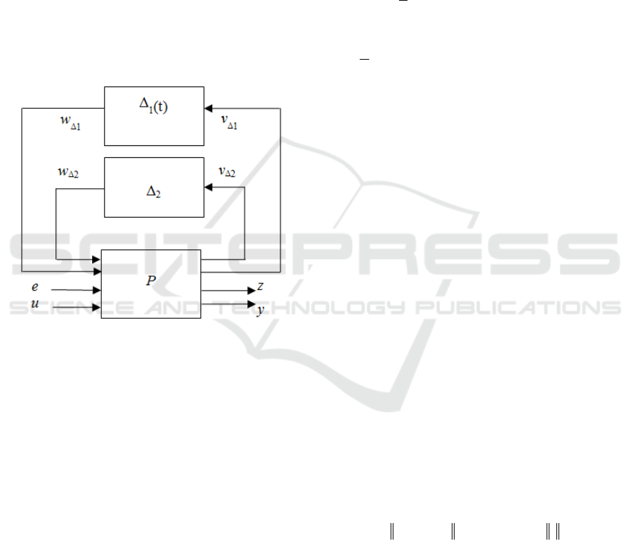
partially known as in Figure 1 where Δ
2
denotes the
unknown part of the uncertainty block and Δ
1
(t)
denotes the well-known part. Because the LFT
modelling framework is common to the LPV/LFT
technic and μ-synthesis technic, some works have
tried to directly merge those two technics leading
generally to the non-convex synthesis problem of
computing the LPV/LFT controller and some
corresponding augmented scalings (Apkarian et al.,
1995) (Blue et al., 1997); thus the problem is usually
addressed using some sub-optimal heuristics
(DeVito et al., 2010) but without guaranty of the
global optimality of the computed LPV controller.
As an alternative to μ-synthesis, the multiple
plants H
∞
-synthesis has emerged and has proved to
be a good compromise between the complexity of
156
Feyel, P.
Evolutionnary Fixed-Structure LPV/LFT Controller Synthesis for Multiple Plants.
DOI: 10.5220/0006858101560165
In Proceedings of the 15th International Conference on Informatics in Control, Automation and Robotics (ICINCO 2018) - Volume 1, pages 156-165
ISBN: 978-989-758-321-6
Copyright © 2018 by SCITEPRESS – Science and Technology Publications, Lda. All rights reserved

the μ-synthesis technic and the conservatism of the
non-structured uncertainty framework (Apkarian,
2002), (Feyel et al, 2014b). Based on the same idea,
we propose in this work to extend the LPV/LFT
synthesis approach to the multiple plants framework;
the main idea is to use the multiple plants framework
instead of μ-technics to make the LPV/LFT
controller be robust against unknown uncertainties.
The paper is composed as follows: in section 2
we recall the basics of the LPV/LFT controller
synthesis problem and the multiple plants extension
is proposed. In Section 3, the perturbed differential
evolution algorithm in described in order to solve
the LPV/LFT problem described in section 4.
Finally an example showing the efficiency of the
method is proposed in section 5
Figure 1: The LFT modelling framework with well-known
(Δ
1
(t)) and unknown (Δ
2
) uncertainty blocks.
2 THE LPV/LFT CONTROLLER
SYNTHESIS PROBLEM
2.1 Notation
First we consider the system in LFT form depicted
in Figure 2a where Δ(t) represent the varying
uncertainties.
()
ez
nn
Rez
×
∈,
refers to the
performance channels.
y
n
Ry ∈
are the measures and
u
n
Ru ∈
is the control signal. P is a LTI plant and we
have:
()
,()
u
ze
FP t
y
u
 
=Δ
 
 
(1)
The uncertainty block Δ(t) is assumed to be block-
diagonal structured:
()
1
1
() () , , ()
n
rnr
t blockdiag t I t I
ΔΔ
Δ= θ θ
(2)
where r
i
>1 when the i
th
time varying parameter θ
i
(t)
is repeated in Δ(t) and:
1
n
i
i
rr
Δ
=
=

(3)
Thus (v
Δ
,w
Δ
) ∈ R
r×r
refers to the uncertainty
channels.
We define Δ as the set of matrices with the same
structure as Δ(t):
()
11
() , , () ,
:.
()
n
rnr
i
diag t I t I
tR
Δ
Δ


θθ


Δ=


θ∈




(4)
2.2 Principle of LPV Synthesis for
Multiple Plants
2.2.1 Basics of the LPV/LFT Controller
Synthesis Problem
To ensure the stability and the performance in the
LPV framework, we seek a controller with the same
parametric dependence as the system to be
controlled. Then the controller will be adjusted
depending on the evolution of time varying
parameters, which are supposed to be measured or
estimated. Thus the controller is a LPV system with
the following form (Apkarian et al, 1995):
()
,()
l
uFK ty=Δ
(5)
where K is LTI. Considering the Figure 2b, the
close-loop between z and e is written:
() ()()()
.)(,,)(,,, tKFtPFFKPT
lul
ΔΔ=Δ
(6)
The problem is to find a LTI controller K which:
- internally stabilizes the closed-loop
T(P,K,Δ) for all uncertainties such as
1)()(
2
≤ΔΔγ tt
T
,
-
()
γ≤Δ
2
,, KPT
, where
2
is the L
2
-
induced norm.
Following the same idea as in (Apkarian et al,
1995), the two schemes depicted in Figure 2b and
Figure 3 are strictly equivalent.
Introducing the new outputs to survey v
k
∈ R
r
, the
new exogenous inputs w
k
∈ R
r
, the new measures y
k
∈ R
r
and the new control signals u
k
∈ R
r
, an
augmented plant P
a
(s) can be defined in (7).
Evolutionnary Fixed-Structure LPV/LFT Controller Synthesis for Multiple Plants
157

















=


























=
















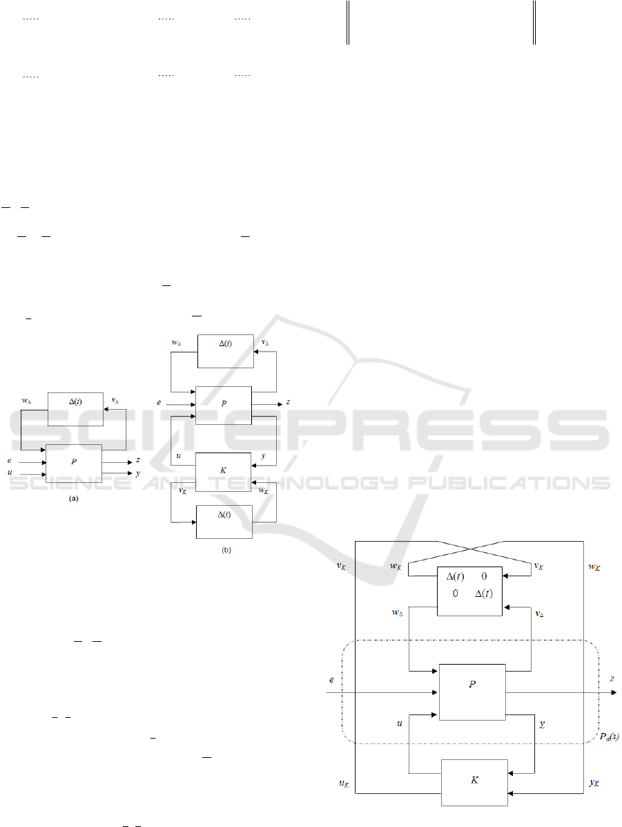
ΔΔΔ
K
K
a
K
K
r
r
K
K
u
u
e
w
w
sP
u
u
e
w
w
I
sP
I
y
y
z
v
v
)(
00
0)(0
00
(7)
Thus, the LPV synthesis problem can be viewed as a
more classical performance robustness one applied
to the nominal plant P
a
(s) towards the uncertainty
block diag(Δ(t),Δ(t)).
In the following, the repeated structure is noted
Δ⊕Δ:
()
{
}
:(),():()blockdiag t t tΔ⊕Δ = Δ Δ Δ ∈Δ
(8)
Now we consider the set of scalings positive definite
associated with the structure Δ:
{
}
0: , R
rr
LL L L
×
Δ
=> Δ=Δ∀Δ∈Δ⊂
(9)
Figure 2: The LFT/LPV model (a) and the LPV closed-
loop scheme (b).
The set of scalings positive definite commuting with
the structure Δ⊕Δ is then defined by:
12
23
13
22
0
,and
,
T
LL
LL
L
LL L
LL
Δ⊕Δ
Δ


>





=


∈


Δ=Δ ∀Δ∈Δ

(10)
According to (Apkarian et al, 1995), F
l
(K,Δ(t)) is a
γ-suboptimal gain-scheduled H
∞
-controller if there
exists a scaling L ∈ L
Δ⊕Δ
and a LTI control structure
K such that the nominal closed-loop system F
l
(P
a
,K)
is internally stable and satisfies:
()
1/21/2
00
,
00
(), ()
ee
zz
nnnn
la
LL
F
II
FFPsKs
−
××
∞

<
γ




 
=
(11)
Assuming that such a controller exists and that:
:
:
y
yy y
y
y
KK
KK
KKK
KK
K
KK
K
AB
K
CD
ABB
DD
C
DD
C
Δ
Δ
ΔΔΔ
Δ

=









=















(12)
Then the gain-scheduled controller F
l
(K,Δ(t)) has the
state-space implementation (13).
()
()
1
''
(): ,():
''
'
'
'
'
() ()
yy
yy
yy y y
KK
l
KK
KKK K
KKK K
KKK K
KK K K
K
AB
KFKt
CD
AABMC
BBBMD
CCDMC
DDDMD
MtIDt
ΔΔ
ΔΔ
ΔΔ
ΔΔ
ΔΔ
Δ
Δ
Δ
Δ
−
Δ

Δ= Δ =


=+
=+
=+
=+
=Δ − Δ
(13)
Figure 3: An equivalent LPV closed-loop scheme.
ICINCO 2018 - 15th International Conference on Informatics in Control, Automation and Robotics
158

2.2.2 The Proposed Multiple Plants
Extension
As said in introduction, we propose to use the
multiple plants framework instead of μ-technics to
make the LPV/LFT controller be robust against
unknown uncertainties. The unknown uncertainties
allow us to define a set of m plants with equation
(14).
{}
misP
i
,,1),( ==℘
(14)
As depicted in Figure 4 and according to the
previous paragraph, F
l
(K,Δ(t)) is a robust γ-
suboptimal gain-scheduled H
∞
-controller if there
exists a scaling L ∈ L
Δ⊕Δ
and a LTI control structure
K such that each closed-loop system
()
(),
i
la
FPsK
is
internally stable and satisfies:
()
1/ 2
1/2
1, ,
00
max
00
(), ()
eezz
i
i
im
nnnn
ila
LL
F
II
FFPsKs
−
=
××
∞




<
γ

 




=

(15)
where each
()
i
a
P
s
is defined by equation (7) with
P
i
(s) instead of P(s).
Figure 4: The multiple plants LPV/LFT controller
synthesis problem.
Due to the complexity of the posed problem, we
propose to use the evolutionary algorithm described
below to solve it.
3 THE PERTURBED
DIFFERENTIAL EVOLUTION
(PDE) ALGORITHM
The Differential Evolution (DE) algorithm (Storm et
al, 1995) is a recent metaheuristic which belongs to
the class of evolutionary algorithms (like genetic
algorithms for instance). Such a stochastic algorithm
is helpful for minimizing a nonlinear function f(X)
whose gradient cannot be computed (for instance if
f(X) is not differentiable) so that classical methods
cannot be used. Here the only requirement is the
capability of evaluating function f(X), called the
fitness. As a main drawback of such a stochastic
algorithm, the result of the optimization problem has
to be considered in a statistical way but a good
solution (that is near the global optimum) is often
found. The reader can have a good introduction of
metaheuristic methods in (Dréo et al, 2006).
3.1 Description
To introduce the DE algorithm, we consider the
problem of finding
opt
X so that
()()
XfX
X
opt
Ψ ∈
= argmin
where Ψ
n
R
⊂ is the search
space for
X.
In the following, rnd(
x,y) designed a random value
generated by a uniform distribution on the interval
[
x, y].
A description of the classical DE algorithm is as
follows.
Step 0: Initialisation
Construct an initial population P with N individuals:
{}
.
1 Ni
,...,X,...,XXP =
(16)
Each individual is defined by its
n genes:
()
.,...,,...,
T
1 inijii
xxxX =
(17)
Thus
n is also the problem dimension.
Assuming that
,
j
j
j
x
xx


∈


, the j
th
component of
the
i
th
individual is randomly chosen in its definition
interval:
()
(0)
rnd
with and
,
1,..., 1,...,
j
ij j
ij
xxx
iNjn
=
==
(18)
Evolutionnary Fixed-Structure LPV/LFT Controller Synthesis for Multiple Plants
159

Now the k
th
iteration consists of the three following
steps.
Step 1: Mutation
Usually two mutation schemes can be considered,
the rand one and the best one, as defined in (19).
(
)
()
)()()(1)(
)()()(1)(
Best
Rand
k
b
k
a
k
best
k
i
k
c
k
b
k
a
k
i
ii
iii
XXFXU
XXFXU
−+=→
−+=→
+
+
(19)
where
iii
cba
X,X,X are different and randomly
chosen in the population and
best
X is the best
individual (with respect to the fitness) since the
beginning of optimisation.
[] 20,∈F is a number
called the mutation factor. At each iteration,
N
mutants
U
i
are defined according to one of these
rules.
Note that usually the rand scheme encourages
diversity whereas the best scheme encourages fast
convergence, but very often to a suboptimal
solution. That is why we propose here to use the
mutation scheme depicted in (20) which is a merge
of the two previous schemes and known as the
“DE/rand-to-best/1” mutation scheme.
()
()
(1) () () ()
() ()
Rand to Best
iii
i
kk kk
ia bc
kk
best a
UXFXX
F' X X
+
→=+ −
+−
(20)
Where
F’∈ [0,2] is another mutation factor.
Finally to avoid stagnation during the optimization
process, we decide to perturb the mutant obtained in
(20) by the rule (21).
(1) (1)
rnd( 1,1)
rnd(0,1)
i
kk
ii d
f
UU X
if p
++
=+−
<
(21)
Where
p
f
is the probability of perturbation and
i
d
X
is different from
iii
cba
X,X,X and randomly chosen
in the population.
Step 2: Cross-over
By crossing-over
() 1+k
i
U
with
() k
i
X
, a new
individual
() 1+k
i
V
is generated with genes defined as
follows:





=≤
=
+
+
else
iforrnd(0,1)if
)(
1)(
1)(
k
ij
irij
k
ij
k
ij
x
jjCu
v
(22)
where
[] 0.90.1,∈
r
C is the crossing-rate and j
i
an
integer number randomly chosen in
{} ,...,N,21 . As
the population moves towards its bounds, the
bounce-back method can be used to generate vectors
that will be located even closer the bounds (Storm
et
al,
1995).
Step 3: Selection
The population is updated with individuals defined
by:
()()



≤
=
++
+
else
if
)(
)(1)(1)(
1)(
k
i
k
i
k
i
k
i
k
i
X
XfVfV
X
(23)
If the stopping criterion is satisfied, then return best
solution found so far, otherwise go to step 1.
The stopping criterion can be:
-
a maximum number of iterations,
-
the convergence of the algorithm which is
detected when all individuals tend to be
similar and centered around the best one,
that is when (24) is verified.
ε<
−
++
=
xx
XX
k
best
k
i
Ni
-
max
)1()1(
,...,1
(24)
3.2 Settings for Control Problems
One of the main advantages of this heuristic
approach is its low number of tuning parameters. In
this work we use the classical values given by
(Storm
et al, 1995) for F and C
r
:
-
The mutation factor: F = 0.75,
-
The cross-over rate: C
r
= 0.8,
A good balance between exploration and
convergence is achieved by enforcing:
F’=1‒F =
0.25.
The mutant is perturbed with a probability
p
f
=
0,025.
The convergence threshold is set by default to:
ε =
0,1%.
Although a population size between 5
n and 10n is
generally advised, we use the same idea as (Clerc,
2012) by setting the size of the population with the
following rule:
(
)
.10floor nN +=
(25)
The number of iterations depends on the problem
and will be specified later and is not very sensitive.
ICINCO 2018 - 15th International Conference on Informatics in Control, Automation and Robotics
160

4 EVOLUTIONNARY FIXED-
STRUCTURE LPV/LFT
SYNTHESIS FOR MULTIPLE
PLANTS
4.1 Notations
Given the controller K with state-space (12) and the
plant
P
a
(s) defined in (26).










=
aaa
aaa
aa
a
a
DDC
DDC
BBA
P
22212
12111
21
:
(26)
The closed-loop
F
l
(P
a
,K) has the following state-
space representation:
()
()
()()
21 2 21
22 2 22
121 21
221
1121 2121
11 12 1 21
11
122222
(), ()
,
cl cl
la
cl cl
aaaka aak
cl
kaa k kaak
aaaka
cl
kaa
cl a a a k a a a k
cl a a a k a
akaa ak
AB
FPsKs
CD
ABMDC BMC
A
B
MC A BMD C
BBMDD
B
BM D
CCDMDCDMC
DD DMDD
MIDD M IDD
−−

=


+

=

+

+

=


=+
=+
=− =−
(27)
We note
λ(A) the set of eigenvalues of A. Then the
close-loop defined in (27) is internally stable iff (28)
holds.
()()()
0realmax <λ
cl
A
(28)
4.2 Fitness Function Definition and
Optimization Scheme
As said before, we propose in that work to use
evolutionary computation to find simultaneously a
structured optimal controller
K and optimal scalings
by solving the following optimization problem:
()
123
,,,
1, ,
min max
,R,1,,
i
i
LL L K
im
la
subject to
LL
F
PK H i m
=
Δ⊕Δ
∞

γ


∈
∈=


(29)
With:
()
1/2
1/2
00
00
(), ()
ee
zz
i
ii
nn
nn
ila
LL
F
II
FFPsKs
−
×
×
∞

γ=






=
(30)
where each
()
i
a
P
s
is defined by equation (7) with
P
i
(s) instead of P(s).
The problem (29) can be rewritten:
;
min ( )
Xxx
f
X

∈

(31)
The unknown X stands for the coefficients of the
state-space matrices (A
k
, B
k
, C
k
, D
k
) of K and for
those of the scalings L
j
(j=1,2,3) which are
symmetric (thus only the upper part of matrices are
searched) and have to commute with Δ.
Note that:
()()
.0min
definitepositivenonsymetric
≥λ−
⇔
M
M
i
i
(32)
Thus:
() () () ()
.0min,min,minmin
31
≥λλλ−
⇔
∉
Δ⊕Δ
LLL
LL
i
i
i
i
i
i
(33)
The fitness function f(X) is given by the evaluation
of the following flowchart:
-
Build (A
k
, B
k
, C
k
, D
k
) from X,
-
Build each
i
cl
A
according to (27) for
i=1,…,m,
-
Build each L
j
(j=1,2,3) from X,
-
Build scaling L from each L
j
according to
(10),
-
Evaluate the global spectral abscissa of the
set of closed-loop plants:
()
()
(
)
1, ,
max max real .
i
cl
im
A
=


λ= λ





(34)
-
According to (33) evaluate:
() () ()
(
)
LLL
i
i
i
i
i
i
λλλ−=λ min,min,minmin
31
(35)
-
If max(
λ
,
λ
) ≥ 0, evaluate:
(
)
,,max)( λλ=Xf
(36)
-
Else :
o Build each
()
(),
i
la
FPsK
according to (30),
Evolutionnary Fixed-Structure LPV/LFT Controller Synthesis for Multiple Plants
161

o Compute each γ
i
according to (30),
o Evaluate :
1, ,
1
() .
max
i
im
fX
=
=−
γ

(37)
As done in (Feyel et al, 2014a) and (Feyel et al,
2014b) to increase the rate of convergence, we use
the tridiagonal form for the state-matrix A
k
(which
limits the number of unknowns) and a
transformation of the search space interval is
performed to increase the sensitivity of the
algorithm.
5 EXAMPLE
5.1 Specification
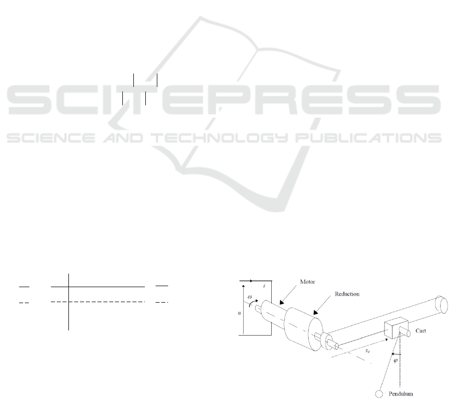
The proposed method has been tested for the
pendulum in the cart depicted in the Figure 5. The
system, denoted H, can be modelled by the
following simplified equations:
() () () ()
() () () () ()
:() ()
() () () () 0
() () ()
c
cl
l
Li t Ri t t u t
J
ttftdt it
r
Hxt t
N
xt vt t g t
vt lt t

++ϕω=

ω+ω+ =ϕ



==ω



++α
φ
+
φ
=

=φ






 

(38)
Where:
-
i(t), u(t) : current, voltage in the motor;
-
ω(t) : rotation speed of the motor;
-
x
c
(t) : position of the cart;
-
φ(t) : angle of the pendulum;
-
d(t) : disturbance torque;
Definitions and nominal values of parameters are
given in Table 2; ϕ(t) and x
c
(t) are measured with
measurement gain k
x
and k
ϕ
.
The specification required is:
-
Tracking the reference defined in Figure 7,
-
No steady-state error, overshoot lower than
0,01 m, |ϕ(t)| < 0,1 rad, time response less
than 6s,
-
|u(t)| < 15 V,
-
Good stability margins.
5.2 Standard H
∞
Synthesis
We consider the H
∞
-control scheme depicted in
Figure 6; it is easy to verify that the following
weights satisfy the specification with the nominal
plant.
1
2
3456
500 866
()
1000 0,866
99,5 200
()
0.995 2000
0,01; 2 ; 0,1; 1
s
Ws
s
s
Ws
s
WWWW
+
=
+
+
=
+
====
(39)
Thus a 3 DOF controller with order 7 is obtained.
The corresponding position response of the cart is
given in Figure 7.
5.3 Standard Polytopic LPV/LFT
Synthesis
In fact two measurable parameters are time varying
in the following intervals:
-
l(t) ∈ [0,1 ; 0,3], the length of the
pendulum;
-
J(t) ∈ [3.10
-6
; 50.10
-6
], the inertia of the
motor.
Typical trajectories for J(t) and l(t) are given in
Figure 8. As we can see in Figure 9, those variations
are disturbing the cart time response and the
previous standard H
∞
controller doesn’t succeed in
stabilizing the time varying plant. Assuming J(t) and
l(t) measurable, we compute a gain-scheduled
controller first using the polytopic approach
(Apkarian et al, 1993) so that the specification
remains satisfied in spite of parameters variations.
Thus we pose as varying parameters:
11
12
() , ()
p
lt p Jt
−−
==
(40)
So that the polytope is defined by:
2-1-6
2
2-1-6
-1
1
-1
.mkg10.333,0.mkg10.02,0
m10m33,3
<<
<<
p
p
(41)
And:
11 112 2 22
12
11 2 2
12
12
12
(1 ) ; (1 )
() ()
;
pp pp p p
ppt ppt
pp pp
=θ + −θ =θ + −θ
−−
θ= θ=
−−
(42)
The polytopic LPV plant is thus on the form:
() ()
()
()
12 1 2 1
12 2
12 2 1 2 12
1
,(1) ,
(1 ) , (1 ) (1 ) ,
LPV
HHpp Hpp
H
pp Hpp
=θ θ + −θ θ
+θ − θ + − θ − θ
(43)
As we can see in Figure 9, the LPV plant is thus
stabilized.
ICINCO 2018 - 15th International Conference on Informatics in Control, Automation and Robotics
162

5.4 Robust Fixed-structure LPV/LFT
Synthesis
In addition of the previous (measured) parameters
variations, the friction coefficient f is also uncertain
(and unmeasured) and can vary in the interval
511
0;13.10 .( . )fNms
−−−

∈

. As we can see in
Figure 10, the cart response is really disturbed and
even the LPV polytopic previous controller doesn’t
succeed in stabilizing the cart. Thus we propose to
use our multiple-plants approach to compute a more
robust LPV controller. We proceed in two steps:
-
The first one consists in modelling the
LPV plant using the LPV/LFT modelling
framework,
-
The second one consists in defining a set
of the previous LPV plants to take into account the
unmeasurable uncertainty.
5.4.1 LPV/LFT Plant Modelling
The first step consists in finding a LFT model for the
uncertain system. For that purpose, we define:
.1)(,
~
)(
~
)()(
~
,1)(,
~
)(
~
)()(
~
~
1
~
0
1
~
1
~
0
1
≤δδ+==
≤δδ+==
−
−
tltltltl
tJtJtJtJ
ll
JJ
(44)
with:
()
()
()
()
11
1minmax
11
0minmax
11
1minmax
11
0minmax
0.5
0.5
0.5
0.5
JJJ
JJJ
lll
lll
−−
−−
−−
−−
=−
=+
=−
=+




(45)
A state-space representation of the uncertain system
with state-vector X(t)=(i(t),ω(t),x
c
(t),ϕ(t),v
l
(t))
T
, is
easily obtained:
ΔΔ
Δ
ϕϕϕδϕ
δ
δδδδδ
δ
Δ
Δ=




























=














ϕ
wtv
u
d
w
X
DDDC
DDDC
DDDC
BBBA
x
v
X
ud
xuxdxx
ud
ud
c
)(

(46)
Where the (measurable) uncertainty block is
structured as follows:
(
)
)(),(),(),()(
~~~~
ttttdiagt
ll
JJ
δδδδ=Δ
(47)
5.4.2 Multiple Plants LPV/LFT Modelling
We propose do define a set of 3 LPV/LFT plants
based on (46) by considering the minimal, nominal
and maximal values of the friction coefficient (48).
{
}
55 11
0 ;6,5.10 ;13.10 .( . )fNms
−− −−
=
(48)
5.4.3 Robust LPV/LFT Controller Synthesis
Now we can compute a 3 DOF controller K with (for
instance) order 4 and symmetric scalings L
j
(j=1,2,3)
commuting with Δ. Thus each of them has the
following block diagonal structure:
{} {}
{} {}
{} {}
{} {}
11 12
12 22
33 34
34 44
00
00
,1,2,3
00
00
jj
jj
j
jj
jj
ll
ll
Lj
ll
ll



==




(49)
Note that searching for diagonal scalings may lead
to too conservative results; but it would be the good
choice if uncertainties were all different (that is not
repeated) in Δ(t).
After proceeding to 10 runs (20000 iterations per
run) on an Intel Core i7-3740 QM – 2.7 GHz
processor and Matlab 2016b, best results are given
in Table 1. We can see that our approach is effective
for a reasonable computing time.
We implement the gain-scheduled controller
according to (13) in Simulink and proceed to a
temporal simulation using references for J(t) and l(t)
defined in Figure 8. As we can see in Figure 10, the
cart response is more robust with our LPV/LFT
(only order 4) controller than with the LPV (full-
order) polytopic controller for different values of the
friction coefficient. Our LPV/LFT controller is
stabilizing and performing for the different f values
whereas the LPV full-order polytopic controller
doesn’t stabilize the plant for f = 0. This makes our
robust fixed-structure LPV/LFT synthesis successful.
Figure 5: Pendulum in a cart.
Evolutionnary Fixed-Structure LPV/LFT Controller Synthesis for Multiple Plants
163

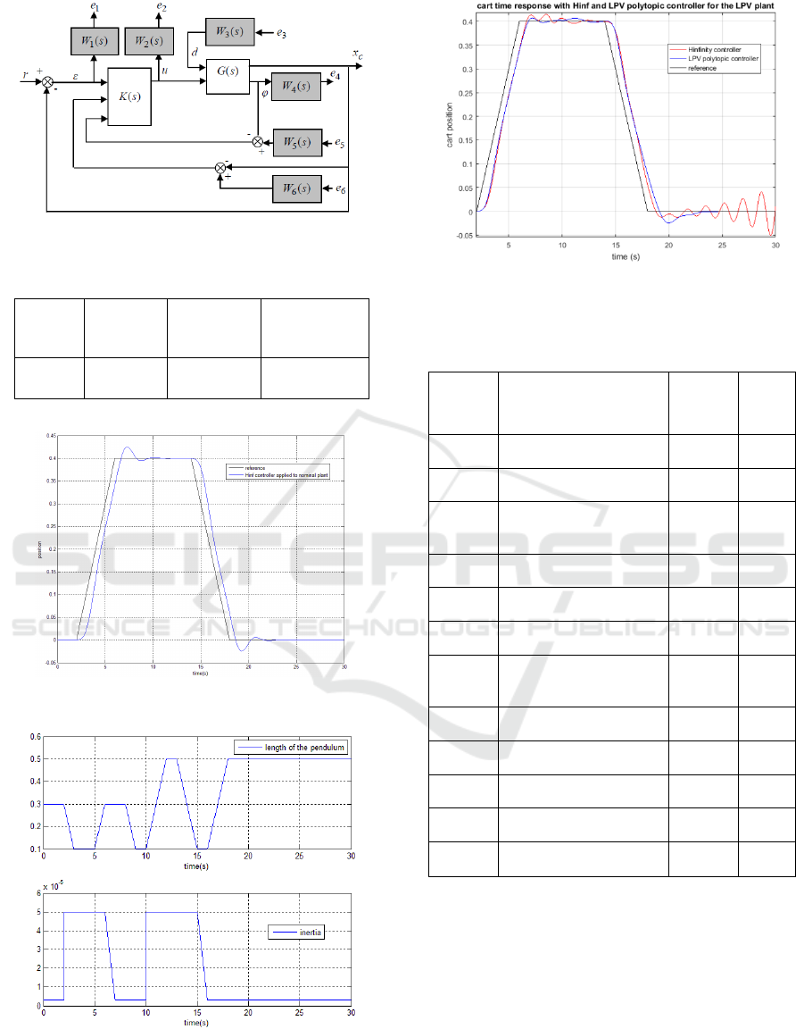
Figure 6: H
∞
control scheme.
Table 1: Results for multiple plants LPV/LFT synthesis.
γ
best
γ
mean
γ
std
t
CPU
/run
(min)
3,39 29,82 25,6 257
Figure 7: H
∞
controller response without uncertainty.
Figure 8: Evolution laws for inertia and length of the
pendulum.
Figure 9: Position reference of the cart and cart responses
when considering the LPV plant.
Table 2: Nominal values of parameters.
Symbol Signification value Unit
R Resistance of the motor 2,3
Ω
L Inductance of the motor 1.10
−3
H
φ
Electromagnetic
constant
0,0162
U.S.I.
f Friction coefficient 6,5.10
-5
N/m.s
-1
r Radius of the pulley 0,022
m
N Gear reduction 17
-
α
Friction coefficient of
the pendulum
0,3
m.s
−1
G Weight acceleration 9,81
m.s
−2
L Length of the pendulum 0,275
m
J Inertia of the motor 5.10
-6
kg.m
2
k
x
Gain of position sensor 39,77
V.m
−1
k
ϕ
Gain of angular sensor 4,77
V.rad
−1
ICINCO 2018 - 15th International Conference on Informatics in Control, Automation and Robotics
164

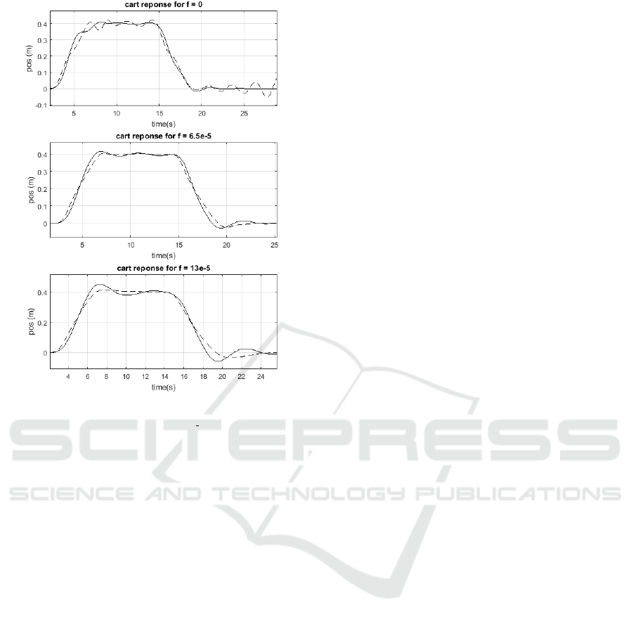
Figure 10: Cart response for different f values: polytopic
approach (--) and proposed approach ( ).
6 CONCLUSIONS
We developed in this paper a method for computing
robust fixed-structure LPV/LFT controllers for
plants with time-varying (measurable) and time
invariant (unmeasurable) uncertainties. By using the
multiple plants framework instead of μ-technics, we
achieved to determine a performing and robust LPV
controller against the unknown uncertainties using
evolutionary computation. Future works deal with
the reduction of computation time.
REFERENCES
Moore, R., Lopes, J., 1999. Paper templates. In
TEMPLATE’06, 1st International Conference on
Template Production
. SCITEPRESS.
Zhou, K., Doyle, J. C., Glover, K., 1996.
Robust and
Optimal Control
. Prentice-Hall.
Apkarian, P., Noll, D., 2002, Nonsmooth H
∞
synthesis. In
Journal of class files, vol.1, n°11.
Young, P., Doyle, J., 1990, Computation of with real and
complex uncertainties. In
Proceedings of the 29th
IEEE Conference on Decision and Control
, pp. 1230-
1235.
Apkarian, P., 2011. non-smooth µ-synthesis. In:
Int.
Journal of Robust and Nonlinear Control
, vol. 21,
Issue 13, pp 1493-1508.
Apkarian, P., Biannic, J.M., Gahinet, P., 1993. Gain
Scheduled H
∞
Control of a Missile via Linear Matrix
Inequalities. In:
Journ. of Guidance Control and Dyn.,
vol. 18, no. 3, pp. 532-538.
Apkarian, P., Gahinet, P., 1995. A Convex
Characterization of Gain-Scheduled H
∞
Controllers.
In:
IEEE Transations on Automatic Control, Vol.40,
N° 5, pp 853-864.
Shi, Y., Tuan, H. D., Apkarian, P., 2010, Nonconvex
Spectral Optimization Algorithms for Reduced-Order
H
∞
LPV-LFT controllers, In: Int. J. Robust. Nonlinear
Control
.
Blue, P. A., Banda, S. S., 1997. D-K iteration with optimal
scales for systems with time-varying and time
invariant uncertainties. In:
Proceedings of the
American Control Conference, Albuquerque, New
Mexico.
De Vito, D., Kron, A., De Lafontaine, J., Lovera, M.,
2010. A Matlab toolbox for LMI-based analysis and
synthesis of LPV/LFT self-scheduled H∞ control
systems. In :
2010 IEEE International Symposium on
Computer-Aided Control System Design.
pp 1397-
1402.
Apkarian. P., 2002. Tuning controllers for multiple models
or operating conditions. In:
http://pierre.apkarian.
free.fr.
Storm, R., Price, K., 1995. Differential Evolution – A
simple and efficient adaptive scheme for global
optimization over continuous spaces. In: Technical
Report TR95 -012, International Computer Science
Institute, Berkeley, California.
Dréo, J., Pétrowski, A., Siarry, P., Taillard, E., 2006.
Metaheuristics for hard optimization, Springer-Verlag,
Berlin.
Clerc, M., 2012. Standard Particle Swarm Optimization,
In :
http://clerc.maurice.free.fr/pso.
Feyel, P., Sandou, G., Duc, G., 2014a. Evolutionnary
Fixed-Structure Mu-synthesis. In:
IEEE Symposium
Series on Computational Intelligence 2014
, Orlando,
Florida, USA.
Feyel, P., Sandou, G., Duc, G., 2014b. Evolutionnary
Fixed-H
∞ synthesis for multiple plants. In: 2014 IEEE
Multi-Conference on Systems and Control, Antibes,
France
.
Evolutionnary Fixed-Structure LPV/LFT Controller Synthesis for Multiple Plants
165