
Analysis of Data Structures Involved in RPQ Evaluation
Frank Tetzel
1
, Hannes Voigt
1
, Marcus Paradies
2
, Romans Kasperovics
3
and Wolfgang Lehner
1
1
Dresden Database Systems Group, Technische Universit
¨
at Dresden, Germany
2
DLR, Jena, Germany
3
SAP SE, Walldorf, Germany
Keywords:
Graph Data Management, Regular Path Queries, Experimental Analysis.
Abstract:
A fundamental ingredient of declarative graph query languages are regular path queries (RPQs). They provide
an expressive yet compact way to match long and complex paths in a data graph by utilizing regular expres-
sions. In this paper, we systematically explore and analyze the design space for the data structures involved
in automaton-based RPQ evaluation. We consider three fundamental data structures used during RPQ pro-
cessing: adjacency lists for quick neighborhood exploration, visited data structure for cycle detection, and the
representation of intermediate results. We conduct an extensive experimental evaluation on realistic graph data
sets and systematically investigate various alternative data structure representations and implementation vari-
ants. We show that carefully crafted data structures which exploit the access pattern of RPQs lead to reduced
peak memory consumption and evaluation time.
1 INTRODUCTION
In recent years, the graph data model had a renais-
sance in the database community, positioning itself as
an alternative to the traditional relational data model.
The interest is mainly driven by novel, emerging use
cases like the analysis of social networks. In such use
cases the relationships between the entities and the-
refore the topology of the graph are as important as
other data attached to the entities.
Major database vendors adopted graph data ma-
nagement and integrated it into their database sys-
tems, e.g., Oracle PGX (Raman et al., 2014) and SAP
HANA Graph (Rudolf et al., 2013). Graph database
systems excel in handling multi-hop relationships be-
tween entities, e.g., multi-hop stakeholder relations-
hips between offshore profits and potential tax eva-
ders. One expressive way to match multi-hop re-
lationships are regular path queries (RPQs) (Wood,
2012). Many declarative graph query languages
have support for RPQs, e.g., SPARQL (W3C, 2013),
PGQL (van Rest et al., 2016), and G-Core (Angles
et al., 2018).
RPQs are a compact way to match long paths in a
data graph which conform to a given regular expres-
sion. The regular expression is defined over the set
of edge labels in the data graph. Additionally, every
label can be reversed which checks for incoming ed-
ges with the label instead of outgoing edges, e.g., ex-
pression ˆlikes checks for incoming edges with la-
bel likes. This type of queries is also called two-way
regular path queries (2RPQs). The concatenation of
all edge labels on a path from the start vertex to the
end vertex has to be in the language of the given regu-
lar expression, otherwise it is not a part of the result
set. The result set is a distinct set of tuples consisting
of the start vertex and the end vertex of each matched
path.
One state-of-the-art way to evaluate RPQs is to
transform the regular expression to an equivalent au-
tomaton and use it to guide the search for matching
paths in the data graph. An automaton consists of
one initial state s and one or multiple final states
f . The states are connected by directed transitions
which have edge labels attached as predicates. Fi-
gure 1b shows an automaton for the regular expres-
sion (likes/hasCreator)+.
The search traverses synchronously the automaton
and the data graph, starting at the initial state and all
vertices if no additional index is available which li-
mits the set of start vertices. The transitions in the
automaton restrict which edges in the data graph can
be followed. The edge labels have to be equivalent.
When the traversal reaches one of the final states in
the automaton, a result tuple is produced, consisting
of the vertex from which the search in the data graph
334
Tetzel, F., Voigt, H., Paradies, M., Kasperovics, R. and Lehner, W.
Analysis of Data Structures Involved in RPQ Evaluation.
DOI: 10.5220/0006860303340343
In Proceedings of the 7th International Conference on Data Science, Technology and Applications (DATA 2018), pages 334-343
ISBN: 978-989-758-318-6
Copyright © 2018 by SCITEPRESS – Science and Technology Publications, Lda. All rights reserved
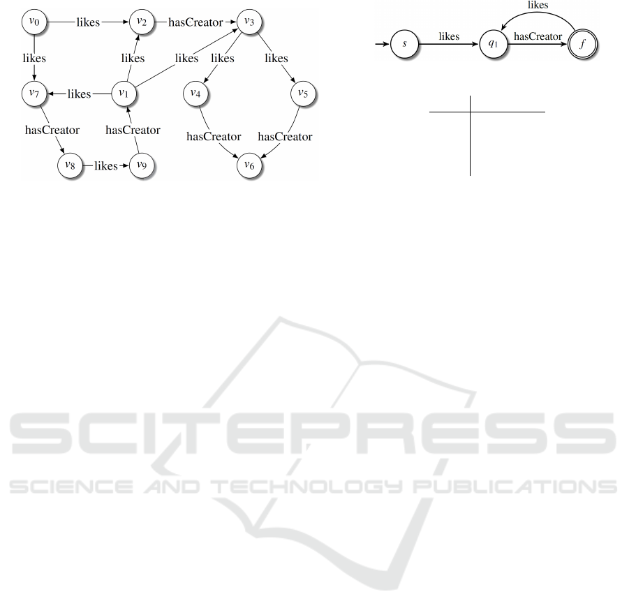
(a) Data graph.
(b) Automaton for (likes/hasCreator)+.
start end
v
0
v
3
,v
6
,v
8
,v
1
v
1
v
4
,v
6
,v
8
,v
1
v
3
v
6
v
8
v
1
,v
8
(c) Result pairs grouped
on the start vertex.
Figure 1: Example for RPQ evaluation.
started and the current vertex when the final state was
reached. Figure 1 shows a small example. The re-
sulting pairs are shown grouped on the start vertex.
Many graph database systems operate purely or
mainly in main memory. One major challenge of RPQ
evaluation in this context is the very high peak me-
mory consumption in many queries, which can easily
lead to slow-downs or out-of-memory situations. Es-
pecially RPQs with unbounded recursions, e.g., with
a Kleene-star, produce large intermediate results, and
also large result sets. To investigate how this memory
consumption can be reduced we study the data struc-
tures involved in the RPQ evaluation, and search for
mitigations and alternatives.
Our contributions in this paper are three-fold:
1. We revisit automaton-based RPQ evaluation, ex-
amine involved data structures, and discuss their
usage in the algorithm. Section 2 outlines the al-
gorithm with the relevant data structures.
2. We provide a detailed discussion of implementa-
tion variants for each involved data structure ai-
ming to lower the memory footprint and improve
the evaluation time. This is described in Section 3.
3. We experimentally evaluate the discussed variants
of the data structures on data graphs of various
sizes and different query sets. Section 4 discusses
the experiments and our findings.
Section 5 examines related work and Section 6 con-
cludes the paper.
2 AUTOMATON-BASED RPQ
EVALUATION
Using an automaton representation of the regular
expression is a state-of-the-art method to evaluate
RPQs. The automaton is used to guide the search for
matching paths in the data graph, similar to a pattern
graph in graph pattern matching. Most often a de-
terministic finite automaton (DFA) is employed as it
has only a single initial state which acts as a natural
starting point for the search. Attached to every state
transition in the DFA is an edge label predicate. It
represents a traversal step in the data graph along an
equivalent edge label. ε-transitions, which have the
empty word as predicate on the transition, are not al-
lowed.
The search has to keep track where it initially star-
ted from as the start vertex is part of the result pairs.
The matched paths are not returned, so it is sufficient
to just track the start vertex. Information to recon-
struct the path is not required. Additionally, the se-
arch has to know the current state in the automaton
and the current vertex in the data graph. Hence, the
search state is a triple (v
s
,s,v
i
) consisting of the start
vertex v
s
, the state s, and the current vertex v
i
.
Let S be the set of all valid start vertices in the
graph. For each v
i
∈ S we have one initial search state
(v
i
,s,v
i
), e.g., in Fig. 1 one initial state is (v
0
,s,v
0
). S
is either given by the user, a nesting query, or includes
all vertices of the graph. All initial search states form
the first intermediate results (IR).
The search proceeds in traversal steps. Each step
transforms search states from IR into new search sta-
tes or drops them. The edges of the current vertex
are examined if they match an edge label predicate
of an outgoing transition of the current state. As is
standard in most graph processing engines, an adja-
cency list (ADJ) is used to provide quick access to all
incoming and outgoing edges of each vertex. Each
match produces a new search state consisting of the
start vertex which is just copied over, the state where
the matching transition leads to, and the vertex where
the matching edge leads to. The new search states are
then checked against a visited data structure (VIS) to
make sure it is a search state which was not seen be-
Analysis of Data Structures Involved in RPQ Evaluation
335
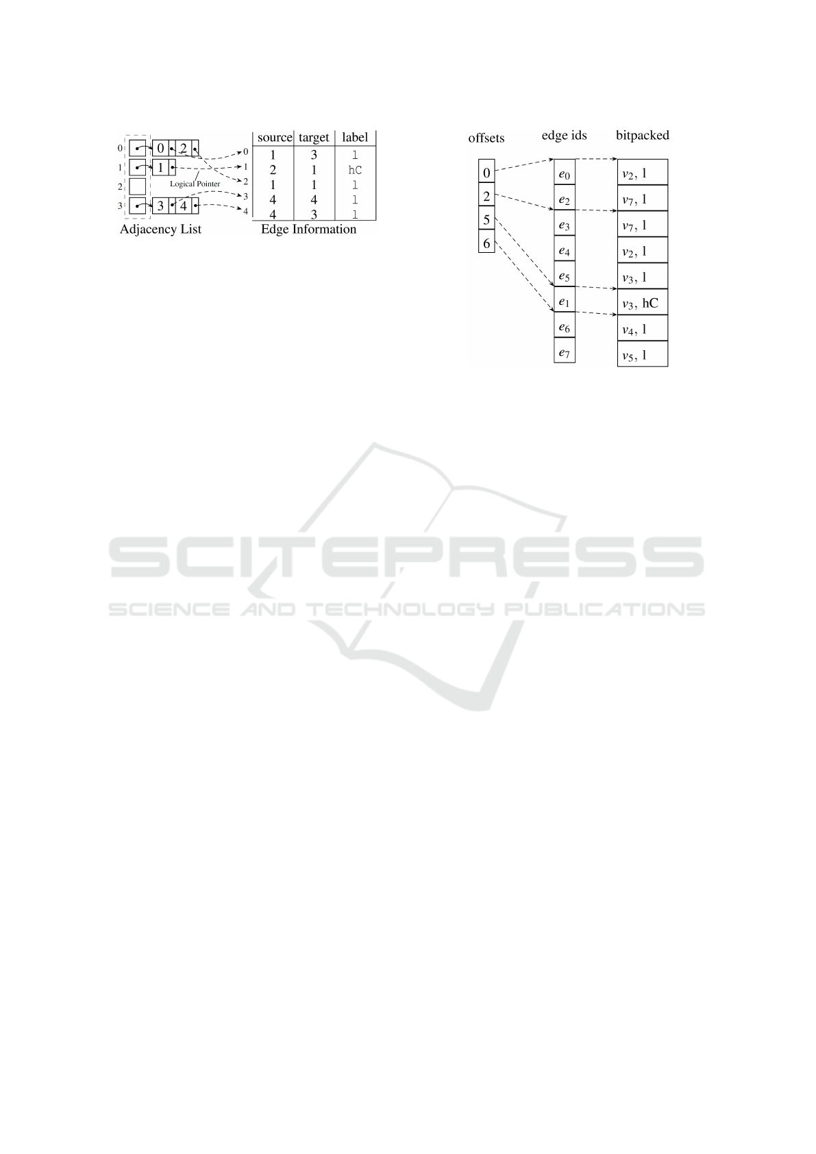
Figure 2: Mutable adjacency list consisting of a two-
dimensional dynamic array with edge identifiers which re-
fer to edge information like source, target and label of the
referenced edge.
fore. If it is new, it is added to IR for the next step
and also to VIS, otherwise it is dropped. In Fig. 1, the
search state (v
0
,s,v
0
) would produce two new search
states (v
0
,q
1
,v
2
) and (v
0
,q
1
,v
7
) as there are two mat-
ching edges leading to v
2
and v
7
which match the only
outgoing transition of the initial state s to the state q
1
.
When the search reaches a final state, a new tuple
for the result set (RS) consisting of the start vertex
and the current vertex is produced, additionally to the
new search state. The search ends when there are no
search states available anymore to explore. In other
words, IR is empty.
The search can be conducted with two diffe-
rent traversal strategies: depth-first search (DFS) and
breadth-first search (BFS). The major difference is
that DFS does not materialize IR and always produ-
ces just one search state, and follows it. It employs
backtracking to reach old search states and produces
the next search states from them. Therefore, DFS is
better suited for memory constraint situations.
3 DATA STRUCTURES
In the following sections, we investigate in detail vari-
ous implementation variants of the data structures for
adjacency list (ADJ), visited (VIS), and intermediate
results (IR).
3.1 Adjacency List
The graph topology is commonly stored in an adja-
cency list to support fast access to adjacent edges and
vertices. All edges have a unique identifier and pro-
vide the information about the edge label, source ver-
tex and target vertex. Vertices have unique identifiers
as well. As edge label predicates can be reversed in
RPQs, the graph traversal has to follow not only out-
going but also incoming edges, from target vertex to
source vertex. Hence, it is common practice to use
two adjacency lists: one containing all outgoing ed-
ges per vertex and one for all incoming edges per ver-
Figure 3: CSR with edge identifiers and CSR with bitpac-
ked values consisting of vertex identifier and label identifier,
both can share the offset array.
tex. In the following, we only discuss each variant for
outgoing edges.
Vectors. A common representation is a two-
dimensional dynamic array which contains edge iden-
tifiers, as illustrated in Fig. 2.
The first dimension is a dynamic array containing
one entry per vertex. Each entry is yet another dyn-
amic array containing all outgoing edges originating
from the corresponding vertex. Edges are represented
with edge identifiers, which can be used to lookup the
edge information.
The use of dynamic arrays allows the insertion and
removal of edges and vertices. The entries in the dyn-
amic array are stored consecutively in memory which
results in good cache locality and, therefore, good
read performance. The name adjacency list might im-
ply the use of linked lists, but the worse read perfor-
mance of linked lists, because of pointer chasing, ma-
kes them a less appealing choice.
CSR. Another widespread representation is the CSR
(compressed sparse row) format. It trades off mutabi-
lity for a more compact and cache friendly represen-
tation. The arrays in the second dimension are col-
lapsed into one single array which then contains one
entry for each edge in the data graph, sorted in such
a way that all outgoing edges of the first vertex are
grouped together at the beginning of the array. There-
after all outgoing edges of the second vertex are sto-
red, then for the third vertex, and so on.
The entries in the first array are offsets into the
second array, marking the beginning of the outgoing
edges for the corresponding vertex. The end is mar-
ked with the beginning for the next vertex. The left
side of Fig. 3 gives an illustration of CSR.
An insertion into a CSR structure is time-
DATA 2018 - 7th International Conference on Data Science, Technology and Applications
336

consuming since it has to shift following existing en-
tries to make space before adding the new entry. The
order of the entries has to be kept. Therefore, CSR is
usually employed when the data graph remains static.
Bitpacked. A CSR format optimized for RPQ evalu-
ation uses bitpacked values instead of edge identifiers.
A bitpacked value combines label and target vertex of
the edge into a single value. It removes the additio-
nal indirection to lookup edge label and target vertex
with the edge identifier. The lookup is in general an
expensive random access with a cache miss which is
avoided by having all the information already in the
adjacency list.
Dictionary-encoded edge labels only require a few
bits to be stored. Bitpacking reserves a fixed number
of low bits for the edge label and encodes the target
vertex identifier in the remaining high bits. For most
data graphs it is possible to use 32-bit value types,
e.g., LDBC scale factor 10 has 29 146 487 vertices and
15 different edge labels, which require 25 bits and 4
bits, respectively.
The array with bitpacked values can replace or
complement the array with edge identifiers in a CSR
structure as shown in Fig. 3. The complementing va-
riant still allows access to further edge data, such as
edge properties, if required, e.g., graph pattern mat-
ching with predicates on edge properties.
Vertical Partitioning. Another well-known variant
of the CSR format is vertical partitioning. Most re-
gular expressions in RPQs use only a small number
of different edge label predicates. Additionally, if one
looks at a single traversal step which corresponds to a
single state transition in the automaton, the number of
edge labels which have to be checked in the adjacency
of a vertex shrinks even more.
This can be exploited by vertically partitioning the
adjacency list by edge label. Each partition contains
only edges of a single label and is represented by a
CSR with target vertex identifiers in the second ar-
ray. Hence, scanning of non-matching edges can be
avoided and all matching target vertices can be easily
extracted.
3.2 Visited
Next to the adjacency list one key data structure for
good performance in RPQ evaluation is VIS, which
keeps track of already discovered search states and
avoids redundant exploration of the same graph regi-
ons. If the data graph and automaton are cyclic, it is
also necessary to guarantee program termination.
The search state consists of the start vertex, the
state in the automaton and the current vertex in the
data graph. We assume for all following variants that
the search state is grouped on the state. Hence, for
each state in the automaton one separate data struc-
ture for VIS is used, storing a tuple consisting of start
vertex and reached vertex.
It is sufficient to only keep track of discovered ver-
tices as we do not store full path information during
the RPQ processing. It is not relevant for the result
over which edge a certain vertex has been reached as
it is essentially only reachability information constrai-
ned by the regular expression.
In the following paragraphs, we introduce four
data structures, which we employed as VIS.
hashset. One obvious choice for VIS is a hashset,
e.g., C++’s std::unordered set. It stores tuples of
vertex identifiers for start vertex and visited vertex.
Since vertex identifiers are 32-bit values, we essenti-
ally store one 64-bit value per entry.
hashmapset. A variation of a single hashset is a
hashmapset which maps each start vertex to its own
hashset of reached vertices. Splitting the hashset into
multiple smaller hashsets reduces the overhead of re-
hashing. It is hard to estimate the size of VIS in ad-
vance, which results in a lot of resizing and, therefore,
rehashing of the hashset. Since rehashing is less ex-
pensive for smaller hashsets, it is beneficial to split
the single hashset.
roaring. Another obvious choice next to hashsets
are bitsets, in case of roaring, a compressed bitset.
The number of possible values for a tuple of start and
reached vertex is too large for a fixed-size bitset. It
requires |V |
2
bits with V being the set of vertices in
the data graph, additionally multiplied by the number
of states in the automaton. For a graph with 3141 713
vertices like LDBC scale factor 1, the required me-
mory has to encompass several terabytes which is un-
reasonable. Hence, we investigated into compressed
bitsets, and settled for the recently proposed Roaring
Bitmap (Chambi et al., 2016; Lemire et al., 2016).
A Roaring Bitmap prunes unset regions in the bitset
very efficiently and still provides fast random access
which is required for the frequent lookups in VIS.
bitset. One simple trick to still make use of a fixed-
size bitset is to treat start vertices separately and unset
the bitset when the traversal for one start vertex is
done and the traversal for the next one starts. That
way, the size of the bitset is limited to the number of
vertices in the graph. One bit per vertex, multiplied by
the number of states in the automaton as we have vi-
sited per state, is an affordable memory size for most
graphs. Unsetting the bitset has to be very fast to not
become the bottleneck during execution. SIMD in-
structions are used to efficiently unset the whole bit-
set. For queries which only visit a small portion of the
graph, we only partially unset the bitset by keeping
Analysis of Data Structures Involved in RPQ Evaluation
337

track of changed words in the bitset.
3.3 Intermediate and End Results
The number of paths matched by an RPQ can be large,
especially for RPQs with unbounded recursions. Ma-
terializing and storing the end result set can already
be challenging. For some queries intermediate results
are even larger than the end result set. Intermediate
results are only materialized during a BFS graph tra-
versal, but not during a DFS traversal. Hence, a DFS
has much lower peak memory consumption for most
RPQs. We briefly introduce two basic data structures
to store the end result set in the following paragraphs.
vector. The simplest data structure to store the end
result set in is a dynamic array, e.g., a C++ std::vector.
It simply stores all tuples in an array of consecutive
memory. One major drawback is the necessary resi-
zing as the result set size is not known in advance.
During resizing more than twice the amount of me-
mory is allocated for a short moment as the data is
copied to the newly allocated memory. Copying a
large amount of data is a costly operation. The use
of overprovisioned allocation, which allocates more
memory than strictly needed, reduces the number of
resizes considerably.
realloc. Another technique to grow a dynamic array
is reallocation. How reallocation works depends on
the used memory allocator. The default allocator in
Linux
1
uses various allocation schemes depending on
the size of the allocation, and this also changes how
reallocation works. We will only discuss the large
allocation scheme as this is used for the large result
sets. When the allocation size is very large (around
128 KiB
2
), the default allocator employs anonymous
memory mapping to allocate memory from the ope-
rating system. In case of a reallocation, the opera-
ting system enlarges the allocated memory without
copying. The operating system can relocate memory
in the virtual address space efficiently by manipula-
ting page table entries.
In addition to the two resizing strategies introdu-
ced above, we investigated various grouping strate-
gies for the intermediate results (IR). IR is conceptual
set of search states which are triples. Storing triples
runs easily out-of-memory for many RPQs. Hence,
we always group on the start vertex and therefore only
have to store a tuple consisting of state and current
vertex. The tuples are stored in a dynamic array which
either utilizes copying or reallocation as resizing stra-
tegy.
1
Other operating systems have similar mechanisms.
2
the threshold is dynamic, see manpage for mallopt()
and parameter M MMAP THRESHOLD for details
Table 1: LDBC social network with various scale factors.
SF1 SF3 SF10
vertices 3 141 713 8 967 247 29 146 487
edges 17 080 008 50 711 019 171 506 420
stategroup. The tuple can be grouped once more,
in this case on state. For each state, we now only
store a simple list of current vertices. We employed an
array with one entry for each state in the automaton.
The number of states is usually small in most RPQs.
The list of current vertices is realized with a dynamic
array utilizing reallocation for resizing. The memory
footprint is reduced considerably as many tuples share
the same state during the traversal of most RPQs.
vertexgroup. Grouping on vertex instead of state
is also possible but gives no benefit for most RPQs.
There are not many vertices in the data graph reached
in the same traversal step in different states, such that
tuples share the same vertex and have different states.
Another problem is the diversity of the reached verti-
ces in one traversal step. An array with one entry per
vertex in the graph would waste a lot of memory. We
used a hash map instead to map the reached vertex to
a bitset which represents the different shared states.
4 EXPERIMENTAL EVALUATION
We experimentally study the impact of the various
data structures described in Section 3 on the LDBC
3
social network graph. We choose three different scale
factors with an increasing number of vertices and ed-
ges (cf. Table 1). By default, we use vertical parti-
tioning for ADJ, bitset for VIS, stategroup for IR and
realloc for RS. In each experiment we only vary one
data structure; all other data structures remain fixed.
Our prototype provides a columnar, dictionary-
encoded storage for the graph data. Edges are sto-
red in an edge table consisting of source vertex, target
vertex, and edge label. Other edge or vertex proper-
ties are not imported as they are not relevant for the
RPQ evaluation. All columns are dictionary-encoded,
i.e., a dense domain of integer values are stored in the
columns. Source and target share a common dictio-
nary for all vertices.
All experiments were conducted on a Haswell
two-socket machine (Intel(R) Xeon(R) CPU E5-2660
v3) running at 2.6 GHz. The machine has 20 cores
(with SMT up to 40 hardware threads) and 128 GB
of RAM. The RPQ evaluation utilizing a depth-first
traversal is trivially parallelized by running up to 40
traversals starting in different start vertices in paral-
3
http://ldbcouncil.org/
DATA 2018 - 7th International Conference on Data Science, Technology and Applications
338

lel. The breadth-first traversal is additionally inter-
nally parallelized.
We define our own set of queries as there is no
benchmark readily available which includes RPQs.
The LDBC benchmarks only consider rudimentary
RPQs: a path of variable length consisting only of
one edge label, e.g., knows+. The queries Q1 − Q4
are larger recursive queries, matching a long, re-
peated path. They exemplify the expressiveness of
RPQs. According to a recent study of SPARQL query
logs (Bonifati et al., 2017) most real world RPQs are
surprisingly simple. That is why we added three ad-
ditional queries, Q5, Q6 and Q7, which are less com-
plex and also have a much smaller result set. The
query set written in the syntax of SPARQL property
paths looks as follows:
Q1 : (likes/hasCreator)+
Q2 : (hasInterest/ˆhasTag/hasCreator)+
Q3 : (likes/isLocatedIn/ˆisLocatedIn/ˆworkAt)+
Q4 : (likes/isLocatedIn/ˆisPartOf/ˆisLocatedIn/ˆstudyAt)+
Q5 : knows+
Q6 : knows/(likes|ˆhasCreator)
Q7 : ˆisLocatedIn/(hasInterest|hasTag)
The first experiments we conducted analyze the diffe-
rent data structures used for ADJ.
4.1 Adjacency List
Time Measurements. We first run the more com-
plex recursive queries Q1 − Q4 on the smallest data
set with scale factor 1 (SF1). Figures 4a and 4b show
our results. All queries have very similar behavior.
The performance of the DFS is not really impacted
by changing the data structure for ADJ which is not
surprising as a DFS reads only one edge from ADJ
and moves forward with it. Avoiding the lookup into
the edge table only gives a very small speedup.
The BFS on the contrary, gets a lot of speedup
from avoiding the additional lookup as can be seen
by the big drop in evaluation time from CSR with
edge identifiers to CSR with bitpacked values. Ver-
tical partitioning gives yet another small boost as all
adjacent vertices with the correct label can be extrac-
ted directly from the data structure without any addi-
tional check.
Another set of experiments was conducted with
different scale factors of the graph (SF1, SF3 and
SF10). As the more complex recursive RPQs Q1 − 4
run out-of-memory for SF10, we opted for the less
complex query Q5 which has a much smaller result
Table 2: Memory consumption in MB of different data
structures for ADJ on the LDBC dataset of various scale fac-
tors.
SF1 SF3 SF10
vectors 143.7 418.1 1385.5
CSR 80.9 238.7 802.6
bitpacked 80.9 238.7 802.6
partitioned 256.8 740.9 2434.8
set with less pressure on the memory system. Figures
4c and 4d show our results.
We observe the same general behavior as in the
previous experiment. Changing the data structure for
ADJ has little to no impact on the runtime of the
DFS traversal. For BFS on the other hand, avoi-
ding the lookup in the edge table gives about a two
times speedup. Vertical partitioning gives again anot-
her boost in performance.
Memory Consumption. We imported the data sets
into the various data structures for ADJ and measu-
red the memory consumption of each data structure
separately. Table 2 summarizes our findings. As one
would expect, the compact format CSR has the smal-
lest memory footprint. The bitpacked values have the
same size as the edge identifiers. Therefore, the whole
data structure requires the same amount of memory.
The mutable adjacency list vectors with dynamic ar-
rays is bigger than CSR because the dynamic arrays
overprovision their internal memory usage. They al-
locate more memory than strictly required by their
content to avoid growing the data structure too often
when new data is inserted. Growing a dynamic array
is an expensive operation.
Vertical partitioning has the worst memory foot-
print. The edges are partitioned per edge label which
requires no additional memory, but the offsets array
which has as many entries as vertices in the graph is
copied per edge label. In most graphs the number of
edges is way bigger than the number of vertices. The
number of distinct edge labels is also small in most
data sets. Therefore, the increased memory consump-
tion is noticeable but bearable considering the benefits
it yields in evaluation time.
4.2 Visited
To evaluate variants of VIS we fixed all other data
structures to the fastest variant, e.g., employing the
vertical partitioned adjacency list, and only varied vi-
sited data structure. Since the BFS and DFS traversal
strategies resulted in very similar behavior, we only
report our findings with the DFS traversal.
Time Measurements. Fig. 5 shows the relative run-
time of each variant, relative to the hashset variant,
in various queries for scale factor 1 and 3. The me-
Analysis of Data Structures Involved in RPQ Evaluation
339
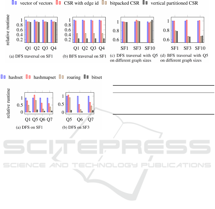
Figure 4: fig:plot-adj-recursive
Figure 5: Relative evaluation time for variants of VIS.
mory consumption, especially for the hashset, was too
big to run the experiments on larger graphs. Complex
queries like Q1 ran out of memory already for scale
factor 3 with the hashset as visited data structure.
The hashmapset gives only a small speedup, and
it heavily depends on the query. It still suffers from
frequent resizing and, therefore, rehashing. As the
hashset also employs overprovisioning, it is not al-
ways better to split it into multiple parts. Q5 shows a
slowdown for hashmapset. Due to overprovisioning,
a large hashset grows faster than many small hashsets
which leads to less frequent rehashing.
Roaring is a promising bitset compression scheme
which works better than hashset and hashmapset. But
again, it heavily depends on the query and which ver-
tices are reached in the traversals. If the vertex iden-
tifiers are nicely clustered together, the compression
and pruning is very efficient in roaring as it relies on
partitioning. A more compact storage leads also to
faster access times.
As obvious from the plots, the fixed-size bitset
with special handling of unsetting is the fastest va-
riant by far, improving evaluation time by a factor of
5 to 14. The bitset fits in both investigated graphs into
the last-level cache which makes the random acces-
ses less costly. The data structure is completely pre-
allocated, i.e., it never has to be resized, which allows
it to reside in the cache for the whole RPQ evalua-
Table 3: Comparison of memory consumption in MB for
VIS across various queries on SF1.
VIS Q1 Q5 Q6 Q7
hashset 34 978.3 3 774.8 9 079.3 135.8
hashmapset 44 570.4 2 562.3 11 063.7 128.3
roaring 2 486.5 80.6 745.1 7.5
bitset 1.2 0.8 1.2 1.2
tion. Additionally, the adaptive strategy for unsetting
exploits the different characteristics of the traversals,
only unsetting changed values when just a few verti-
ces got visited and utilizing vector instructions when
a lot of vertices got visited.
Memory Consumption. To explain the considera-
ble runtime difference we measured the memory con-
sumption of each data structure for various queries.
Table 3 shows the results of our experiment. The me-
mory consumption heavily depends on the query and
how many vertices the graph traversal visits. Query
Q1 produces a large result set and visits a big portion
of the graph. Therefore, all visited data structures re-
quire a lot of memory compared to the other queries,
except bitset. It has a fixed size: as many bits as there
are vertices in the data graph, multiplied by the num-
ber of states in the automaton. It does not depend on
the query.
The bitset is also way smaller than all other data
structures as it is only used for one start vertex and
then unset for the next. All other visited data structu-
res have the problem of a huge input domain they have
to cover. Every vertex in the graph can potentially be
a start vertex, and every vertex could be reached from
each start vertex. Additionally, a separate visited data
structure is required per state in the automaton.
Most queries have a considerably smaller number
of reached vertices and therefore only a sparse num-
ber of entries to store in VIS. The use of a compact
data structure like roaring bitmaps has a lot of bene-
fits. It stores sparse data efficiently in memory and the
previous experiment showed that it still provides fas-
ter access to the data than the hash-based containers.
DATA 2018 - 7th International Conference on Data Science, Technology and Applications
340
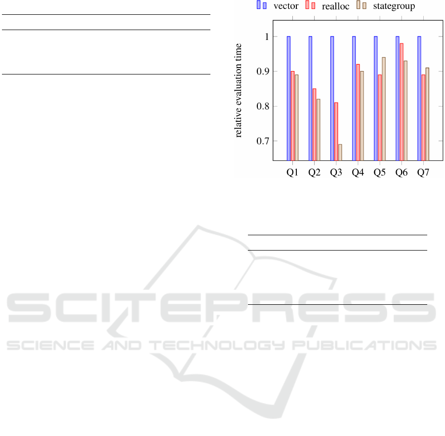
Table 4: Varying return type on SF1 with different queries.
result size vector[ms] realloc[ms] speedup
Q1 79 438 658 10 881.0 5 780.0 1.88
Q5 96 353 856 7 222.7 925.2 7.81
Q6 373 252 434 25 717.8 1 460.9 17.6
Q7 761 791 89.1 71.0 1.25
In the end the best choice for the visited data struc-
ture is the bitset. It has by far the lowest memory
footprint and also provides the fastest evaluation time.
The only limitation is that it can only be used by one
start vertex at a time.
4.3 Intermediate and End Results
We first run a simple experiment where we only vary
the return type. The goal is to see the impact reallo-
cation can have when materializing a large result set.
We used the DFS graph traversal so that no interme-
diate results are materialized.
Time Measurements. Table 4 summarizes our fin-
dings for scale factor 1. The speedup achievable by
employing reallocation instead of copying greatly de-
pends on the result size which has to be materialized.
Copying gets more and more expensive with a larger
amount of entries. With reallocation, the operating
system kernel only has to relocate all memory pages
which make up the dynamic array in the worst case.
A very cheap operation compared to copying. Larger
scale factors did not provide any new insights which
is why we omitted them here.
Memory Consumption. Using a different resizing
strategy does not change the memory consumption as
both data structures employ overprovisioned allocati-
ons in the same way.
The second experiment we conducted focuses on
IR. We use the BFS graph traversal as DFS does not
materialize IR. For the result set we use reallocation
as it was consistently faster in the first experiment.
Time Measurements. Utilizing reallocation for IR
gives consistently a small speedup as is shown in
Fig. 6. The difference is small as IR is not resized of-
ten. When the frontier of the BFS traversal gets larger,
IR also has to get larger, but the size is not decreased
for a small frontier. It stays at the large size.
Grouping the tuple additionally on state (state-
group) gives another speedup in most queries. Many
entries in IR share the same value for state and can
therefore benefit from grouping as less data is stored.
The grouping operation increases the code complex-
ity of the data structure and adds runtime overhead to
the access method. Therefore, not all queries show
an improved runtime. It depends on how many en-
tries share the value the grouping operation works on.
Figure 6: Relative evaluation time for intermediate repre-
sentations.
Table 5: Memory consumption of variants for IR.
vector realloc stategroup
Q1 2 097 152 2 097 152 1 122 304
Q2 16 777 216 16 777 216 8 658 944
Q5 131 072 131 072 73 728
Q6 4 194 304 4 194 304 2 113 536
Q7 1 572 864 1 572 864 892 928
Grouping on vertex (vertexgroup) instead of grouping
on state, was consistently four times slower in each
query which is why we omitted it from the plot. Not
many entries in IR share the same vertex in different
states and rehashing of the employed hash map crea-
ted a performance bottleneck.
Memory Consumption. Table 5 shows the memory
consumption of the variants of IR. vertexgroup is
omitted as the employed hash map used too much
memory to be competitive to the non-grouping tu-
ples. vector and realloc both simply store tuples in
the same format, only the resizing strategy is diffe-
rent. Hence, both data structures have the exact same
memory consumption.
stategroup uses considerable less memory than
vector and realloc as a lot of entries in IR share the
same state. The grouping removes the redundant
storage of state and reduces the memory consump-
tion consistently by a factor of two. Therefore, it is
advisable to always group IR on state.
4.4 Discussion
The adjacency list is a key data structure which is fre-
quently accessed in the RPQ evaluation and a lot of
other graph algorithms. Specialization for the access
pattern during RPQ evaluation resulted in a conside-
Analysis of Data Structures Involved in RPQ Evaluation
341

rable speedup. RPQs consist only of edge label pre-
dicates, so it is advisable to integrate edge label in-
formation into the adjacency list. We exemplified it
by using bitpacked values in the adjacency list, con-
sisting of the edge label and the vertex identifier of
the adjacent vertex. We showed that this approach re-
duces the evaluation time considerably by having the
same memory footprint as an adjacency list with edge
identifiers. Vertical partitioning of the adjacency list
provides even more runtime improvements, but requi-
res also more memory.
For the visited data structure, we found that a
fixed-size bitset with a specialized way for unsetting
all bits gives the best results. It provides the fastest
evaluation time and smallest memory footprint. The
only limitation is that it can only be used by a single
start vertex at the time.
Roaring bitmaps provide a nice alternative when
the traversal should start from multiple start vertices
at the same time. It stores sparse data considerably
more efficiently in a compact data structure compared
to hash-based containers like a hashset. Therefore, the
memory footprint is smaller and the evaluation time
does not suffer from the compact storage as it still
provides fast random access.
Reallocation is a preferable resizing technique for
intermediate results and for the result set. It is con-
sistently faster than copying and avoids sharp spikes
in the memory consumption. Grouping of intermedi-
ate results on the automaton state results in considera-
ble smaller memory consumption and a small speedup
compared to the handling of tuples.
5 RELATED WORK
The broad applicability of RPQs has spurred the de-
velopment of various extensions to the class of 2RPQ
queries (Calvanese et al., 2000; Deutsch and Tannen,
2002). PGQL (van Rest et al., 2016) supports arbi-
trary predicates on any attribute of an edge or vertex
along the path, not just edge label equivalence. G-
Core (Angles et al., 2018) goes one step further with
existential subqueries on sub-branches of the mat-
ching path.
Conjunctive regular path queries (CRPQs) com-
bine several RPQs to a more complex pattern mat-
ching query. Since the general data access patterns
to the underlying data structures are the same as for
2RPQs, we focus in our analysis on the less complex
2RPQs without conjunctions of multiple RPQs.
Extended conjunctive RPQ (ECRPQ) (Barcelo
et al., 2010) extends 2RPQs further by allowing
access to the matched paths as a result, instead of just
pairs of vertices. The added functionality comes at
the expense of making ECRPQs computationally in-
tractable, which is typically not desirable for practical
graph query languages. Therefore, we omit ECRPQs
and paths as a result type from our analysis.
Naturally, the performance of RPQs is sensitive
to the order in which parts of the RPQ are evaluated,
effectively providing an opportunity for query opti-
mization. An interesting approach are so-called rare
labels, i.e., edge labels appearing only seldom on ed-
ges in the data graph (Koschmieder and Leser, 2012).
Rare labels are used to split the regular expression
into subexpressions, which can be evaluated indepen-
dently using a bidirectional BFS traversal. Finally, all
partial solutions are combined into the final result set.
Since rare labels are an optimization technique, they
are orthogonal to our study of data structures for RPQ
evaluation.
WAVEGUIDE (Yakovets et al., 2015) provides
another technique to speedup RPQ processing by in-
troducing waveplans, which allow changing the eva-
luation direction in each traversal step. WAVEGUIDE
supports the materialization of intermediate results
(subexpressions) through views, which can be reused
in the query, e.g., a transitive closure over a path seg-
ment. Both techniques employed by WAVEGUIDE—
match ordering and views—are orthogonal to the
choice of data structures used for RPQ evaluation.
EmptyHeaded (Aberger et al., 2016) introduced
an adaptive adjacency list handling density skew. The
degree of a vertex can vary by a large margin, espe-
cially in social graphs which usually contain super-
nodes. The layout of the list of adjacent vertices is
chosen according to the degree and picks either a sim-
ple array layout or a compact bitset layout.
6 CONCLUSION
We systematically investigated variants of the data
structures involved in the evaluation of RPQs. Care-
fully crafted data structures specialized for their use in
RPQ evaluation showed considerable runtime impro-
vements and decreased memory consumption compa-
red to general purpose data structures.
It is advisable to integrate the edge label infor-
mation into the adjacency list as the RPQ evalua-
tion accesses label information very frequently. In
the form of bitpacked values, it leads to considerable
runtime improvements and no increased memory con-
sumption. Vertical partitioning of the adjacency list
results in even better runtime performance, but requi-
res also additional memory. Another specialization is
grouping on common values in the intermediate re-
DATA 2018 - 7th International Conference on Data Science, Technology and Applications
342

presentation, e.g., grouping on the state of the auto-
maton reduces the memory consumption by half and
results additionally in a small runtime improvement
as less data must be written and read. Reallocation
also avoids spikes in the memory consumption and
therefore reduces peak memory consumption consi-
derably.
In the future, we want to investigate how succinct
data structures affect RPQ evaluation. They are ex-
pected to trade off evaluation time for a very com-
pact representation, e.g., the K
2
-Tree (Brisaboa et al.,
2009), which is a compact adjacency representation.
Another direction we would like to study is the use of
bidirectional traversal instead of unidirectional DFS
and BFS, especially how to detect that both directions
meet each other and how it influences the choice of
intermediate representations. Furthermore, omitting
the check against VIS in some states of the automaton
is an interesting algorithmic variation. Depending on
the query and the data graph it can lead to reduced
memory consumption as less data has to be stored in
VIS, but also to multiple explorations of the same se-
arch states and therefore increased evaluation time.
REFERENCES
Aberger, C. R., Tu, S., Olukotun, K., and R
´
e, C. (2016).
EmptyHeaded: A Relational Engine for Graph Pro-
cessing. In Proceedings of the 2016 International
Conference on Management of Data, SIGMOD ’16,
pages 431–446, New York, NY, USA. ACM.
Angles, R., Arenas, M., Barcel
´
o, P., Boncz, P. A., Fletcher,
G. H. L., Gutierrez, C., Lindaaker, T., Paradies, M.,
Plantikow, S., Sequeda, J., van Rest, O., and Voigt,
H. (2018). G-CORE: A Core for Future Graph Query
Languages. In SIGMOD’18.
Barcelo, P., Hurtado, C., Libkin, L., and Wood, P. (2010).
Expressive Languages for Path Queries over Graph-
structured Data. In PODS ’10, pages 3–14.
Bonifati, A., Martens, W., and Timm, T. (2017). An Analy-
tical Study of Large SPARQL Query Logs. PVLDB,
11(2):149–161.
Brisaboa, N. R., Ladra, S., and Navarro, G. (2009). k2-
Trees for Compact Web Graph Representation. In
Karlgren, J., Tarhio, J., and Hyyr
¨
o, H., editors, SPIRE,
volume 5721 of Lecture Notes in Computer Science.
Springer.
Calvanese, D., De Giacomo, G., Lenzerini, M., and Vardi,
M. Y. (2000). Containment of Conjunctive Regular
Path Queries with Inverse. In KR’00, pages 176–185.
Chambi, S., Lemire, D., Kaser, O., and Godin, R. (2016).
Better bitmap performance with Roaring bitmaps. pa-
ges 709–719.
Deutsch, A. and Tannen, V. (2002). Optimization Properties
for Classes of Conjunctive Regular Path Queries. In
Database Programming Languages, pages 21–39.
Koschmieder, A. and Leser, U. (2012). Regular Path Que-
ries on Large Graphs, pages 177–194.
Lemire, D., Ssi-Yan-Kai, G., and Kaser, O. (2016). Con-
sistently faster and smaller compressed bitmaps with
Roaring.
Raman, R., van Rest, O., Hong, S., Wu, Z., Chafi, H., and
Banerjee, J. (2014). PGX.ISO: Parallel and Efficient
In-Memory Engine for Subgraph Isomorphism. In
GRADES’14, pages 5:1–5:6.
Rudolf, M., Paradies, M., Bornh
¨
ovd, C., and Lehner, W.
(2013). The graph story of the sap hana database. In
BTW, volume 214 of LNI, pages 403–420.
van Rest, O., Hong, S., Kim, J., Meng, X., and Chafi, H.
(2016). PGQL: A Property Graph Query Language.
In GRADES’16, pages 7:1–7:6.
W3C (2013). SPARQL 1.1 Overview. http://www.w3.org/
TR/2013/REC-sparql11-overview-20130321/.
Wood, P. T. (2012). Query Languages for Graph Databases.
SIGMOD Rec., 41(1):50–60.
Yakovets, N., Godfrey, P., and Gryz, J. (2015). WAVEG-
UIDE: Evaluating SPARQL Property Path Queries. In
EDBT’15, pages 525–528.
Analysis of Data Structures Involved in RPQ Evaluation
343
