Use of the Sinusoidal Predictor Method within a Fully Separated

Modeler/Solver Framework for Fast and Flexible EMT Simulations

Pierre-Marie Gibert

, Romain Losseau

, Adrien Guironnet

, Patrick Panciatici

Damien Tromeur-Dervout

and Jocelyne Erhel

System Expertise Department, RTE, Versailles, France

Institut Camille Jordan, University Claude Bernard Lyon 1, Lyon, France

Fluminance Team, Inria Rennes, Rennes, France

Keywords:

Electromagnetic Transients, Time-domain Simulations, Adaptive Step Size Algorithm.

Abstract:

In order to help the introduction of renewable energy sources into the power system, transmission system

operators need extremely reliable simulation tools. In most of the existing simulation tools, heuristics used to

accelerate the simulations combine the modeling and solving aspects. Such kinds of approaches lead to results

whose validity can be questioned. In contrary, our framework aims at avoiding such heuristics by completely

separating the modeler and the solver. However, such an approach is difﬁcult as the computational cost may

be signiﬁcantly higher. In addition, as we simulate the full-waveform of AC power systems, the time step

size used by classical methods for integrating the arising systems of DAE is limited by the frequency of some

electrical components. This is why we developed an efﬁcient solver based on the reference solver SUNDIALS

IDA which takes into account the guessed sinusoidal behavior of the solution oscillating parts in order to

lower the number of iterations for performing a simulation. Our ﬁrst results seem to indicate that the proposed

solver enables to use much larger time steps than a standard integration scheme, while preserving a very high

ﬂexibility of modeling.

1 INTRODUCTION

Modern power systems are characterized by the de-

velopment of smart-grids and the increasing propor-

tion of renewable energy sources in the energy mix.

Therefore, more and more new smart controls and po-

wer electronics devices are introduced into the trans-

mission grid. In order to support this technological

changes while providing a constant security of sup-

ply to their customers, transmission system opera-

tors (TSOs) perform numerous time-domain simula-

tions. Time-domain simulations generally consist in

studying the dynamical behavior of the power system

when it is subject to scenarios, which can be roughly

seen as sequences of discrete events associated with

perturbations and parades.

However, these simulations require important

computational resources because of the stiffness of

the differential algebraic equations (DAE) systems

that arise when modeling power systems in the time-

domain. Indeed, on the one hand, modern com-

ponents introduce electromagnetic transients (EMT)

phenomena, whose typical time range varies from

the microsecond to a few milliseconds. On the ot-

her hand, historically present electrical components

such as synchronous machines lead to electromecha-

nical transients, whose typical time range varies from

the millisecond to the minute. In addition, electro-

mechanical components can be dramatically affected

by electromagnetic phenomena (e.g. magnetic satura-

tion of the coils in synchronous machines). Then, the

study of these two kinds of phenomena can be less

and less separated.

Historically, as the time and space propagation

of EMT through the transmission grid was assumed

to be very limited, simulations were done only on a

small part of the system and during very short time

intervals. This resulted to the use of different mo-

dels and so of different simulation tools depending

of the dynamics to study. The simulation of electro-

magnetic transient phenomena was based on so-called

EMT models. And the simulation of electromechani-

cal transient phenomena was done from so-called TS

(for Transient Stability) models. On the contrary, as

Gibert, P-M., Losseau, R., Guironnet, A., Panciatici, P., Tromeur-Dervout, D. and Erhel, J.

Use of the Sinusoidal Predictor Method within a Fully Separated Modeler/Solver Framework for Fast and Flexible EMT Simulations.

DOI: 10.5220/0006860400340043

In Proceedings of 8th International Conference on Simulation and Modeling Methodologies, Technologies and Applications (SIMULTECH 2018), pages 34-43

ISBN: 978-989-758-323-0

EMT models are more detailed and so contain TS mo-

dels in some ways, our objective is to perform mid-to-

long-term simulations of large-scale power systems

with full-EMT models.

In addition, in most of the existing simulation

tools, the modeling and solving aspects are generally

combined. Indeed, components are directly imple-

mented in discretized form: trapezoidal formula for

smooth dynamics and backward Euler formula for

discontinuities. Although it enables faster computati-

ons, such an approach leads to an increasing number

of heuristics in models and consequently to simulati-

ons whose reliability can be questioned. To ﬁnish, the

DAE systems are generally solved with ﬁxed step size

integration schemes. Therefore, in order to meet some

accuracy requirements, the time step is ﬁxed to very

small values (e.g. 10 µs), which completely prevents

from long-term simulations.

For performing reliable long-term time-domain si-

mulations of power systems represented with EMT

models, our strategy is based on two cornerstones:

1. Completely separating the modeler and the sol-

ver. From a mathematical point of view, the idea

is that the modeler should only build the DAE sy-

stem to solve, which is written in implicit form

i.e. F(t, X,

X) = 0. Then, the solver should per-

form the numerical integration of this system.

2. Integrating the DAE with an adaptive step size

solver. By this way, the time step size is adjus-

ted in order to meet a tolerance target, which ﬁ-

nally reinforces the reliability of the simulation re-

sults. Furthermore, the step size adjustment ena-

bles to possibly optimize the computational cost.

Indeed, as the step size is directly linked to the

dynamics of the solution (the faster its variations,

the smaller the step size), it enables to catch fast

transient phenomena when the system is subject

to perturbations while reducing the computational

cost when the system returns to steady-state.

However, in EMT simulations, using an adaptive

step size strategy is generally inefﬁcient because of

the sinusoidal behavior of the simulated three-phase

voltages and currents. Indeed, their frequency limits

the time step size that is used for the integration. To

tackle this constraint, most of the existing approaches

consist in rewriting the DAE system in order to lower

the frequency of the computed solution. For instance,

in Dynamic Phasors (Demiray, 2008)-(Demiray et al.,

2007) the oscillating components are represented by

their envelope instead of their waveform. Then, as the

frequency of the resulting variables is close to zero,

much larger time steps can be used. However, as this

approach directly affects the model by modifying the

equations to solve in a non strictly equivalent way, it

is not adapted to our framework.

Hence, the method that we implemented takes

into account the sinusoidal behavior of the oscillating

components in the solver. Basically, the idea is to de-

compose the solution as the sum of a periodic part

and a correction term. The former is updated using

parametric estimation. The latter is integrated using

an adaptive step size solver. In previous publicati-

ons, results were obtained with Scilab (Scilab et al.,

2012), a Matlab-like language, which is not suited to

large-scale tests. In this paper, we present the ﬁrst

results obtained with the implementation of our met-

hod into the reference solver SUNDIALS IDA (Hind-

marsh et al., 2005). In order to set our simulations,

we used Dynamo (Guironnet et al., 2018), which is a

simulation engine based on the OpenModelica (Fritz-

son et al., 2006) environment and developed by RTE

for time-domain simulations.

This paper is structured as follows. In the second

section, the mathematical problem to solve when con-

sidering EMT simulations is introduced. In the third

section, our numerical method is presented. In parti-

cular, we detail its implementation into the reference

solver IDA and its interface with Dynamo. In the

fourth section, some numerical results on two power

systems are presented. The ﬁfth section concludes

this paper.

2 MATHEMATICAL PROBLEM

TO SOLVE

In EMT simulations, the mathematical problem to

solve is a set of differential-algebraic equations,

which can be written in its most general form as

F(t, X(t),

X(t)) = 0 (1)

Let d be the dimension of the system. In this equa-

tion t ∈ R, X : R → R

and F : R × R

× R

→ R

In this paper, we present our method for such impli-

cit DAEs. Our previous paper (Gibert et al., 2018)

focuses on semi-explicit DAEs, as DAE systems can

generally be rewritten in such form for most of the

power system applications (Astic et al., 1994).

Furthermore, the solution of this system X is as-

sumed to contain both oscillating (for instance, the

three-phase currents and voltages) and non-oscillating

components, i.e.

X(t) =



(t)



(2)

where X

and X

respectively refer to the oscillating

components and to the non-oscillating components.

Use of the Sinusoidal Predictor Method within a Fully Separated Modeler/Solver Framework for Fast and Flexible EMT Simulations

Let d

(respectively d

= d − d

) be the number of

oscillating (respectively non-oscillating) components

and I

(respectively I

) the associated set of index.

These index sets are known a priori (e.g. network

voltages and currents).

The idea of the Sinusoidal Predictor Method

(SPM) is to take advantage of the behavior of the os-

cillating components in steady-state. Indeed, AC po-

wer systems are designed such as voltages and cur-

rents are as close as possible to balanced three-phase

quantities oscillating at the reference frequency (for

instance 50 Hz for the Continental Europe). In other

words, its means that three-phase systems should ve-

rify:

s,∞

(t) ≈





∞

cos(ω

t + φ

∞

)

∞

cos(ω

t + φ

∞

−

2π

)

∞

cos(ω

t + φ

∞

2π

)





(3)

Where A

∞

and φ

∞

are respectively constant ampli-

tude and phase. In addition, non-oscillating compo-

nents should be constant by deﬁnition, which means

that

ns,∞

≈ 0. Then, in steady-state, the DAE system

should verify





s,∞

(t)

ns,∞





s,∞

(t)



= 0 (4)

Therefore, the SPM, presented in (Gibert et al.,

2017) and (Gibert et al., 2018), consists in decompo-

sing the solution for each time interval [t

, t

n+1

] as the

sum of a periodic part and a correction term, i.e.

X(t) =

(t) + δ(t) (5)

In this equation,

(t) refers to the periodic part of

the solution which corresponds to the guessed steady-

state behavior of the oscillating components. Then, as

mentioned in (3), these variables should be sinusoid

oscillating at the reference frequency i.e.

s,n

(t) = u

sin(ω

t) + v

cos(ω

t) (6)

where ω

= 2π f

is the nominal pulsation (with f

50Hz e.g.). Hence, u

and v

are the Fourier coef-

ﬁcients associated to the fundamental mode f

. The

objective of the SPM is to catch as much as possi-

ble the simple sinusoidal behavior of the solution into

this periodic part. Indeed, as the power system is de-

signed to generate balanced three-phase signals, the

oscillating components of the solution should be si-

nusoids with constant amplitude and phase in steady-

state. So, the f

oscillation ﬁnally corresponds to a

trivial dynamical component of the solution which is

paradoxically the main limit to solver performances

since it constrains the usable step size. The Fourier

coefﬁcients are updated with a parametric estimator

which takes advantage of the property (4).

Therefore the other part of the solution, that we

refer as the correction term, enables to catch transient

parts of the solution that are mainly introduced by dis-

crete events. For instance, it can be envelope vari-

ations (as the Fourier coefﬁcients are set to constant

values for each time interval) or more complex dyn-

amics such as harmonics and offsets. This correction

term is computed by integrating the equations rewrit-

ten on it.

Then, an iteration of the SPM simply consists in

(see ﬁgure 1):

1. ﬁxing the parameters of the periodic part;

2. integrating the equations rewritten on the cor-

rection term;

3. deducing the global solution from the current pe-

riodic part and the integrated correction term;

4. updating the periodic part, by estimating its para-

meters.

1 – Time step

initialization

2 – Correction

term

integration

3 – Global

solution

update

4 - Fourier

coefficients

estimation

"#$

% &

"'(

% )

"'(

% &

"'(

% *

"'(

% .

"'(

)

Figure 1: Overall view of an SPM iteration.

3 PROPOSED SOLVER: IDASPM

3.1 Existing Reference Solver: IDA

IDA is the implicit differential algebraic equations

solver from the SUNDIALS library (Hindmarsh et al.,

2005), developed and still maintained by Lawrence

Livermore National Laboratory. It is a modern ver-

sion of the solver DASSL (Petzold et al., 1982),

which is an industrially validated implementation of

the adaptive step size BDF (Brayton et al., 1972). The

adaptive step size BDF of order q consists in substi-

tuting the time derivative of the solution by the follo-

wing approximation:

n+1

≈

∑

i=0

n,i

n+1−i

(7)

SIMULTECH 2018 - 8th International Conference on Simulation and Modeling Methodologies, Technologies and Applications

where h

= t

n+1

−t

. Then, by injecting this discreti-

zation of

n+1

into (1), the solution at next time step

n+1

can be obtained by solving the following ﬁxed-

point problem:

G(X

n+1

) = F



n+1

, X

n+1

n,0

n+1

+ β



(8)

where β

∑

i=1

n,i

n+1−i

corresponds to the

predicted part of the time derivative of X

n+1

. Then,

the Jacobian of this residual function is given by

n+1

) =

∂F

∂X

n,0

∂F

∂

(9)

More details on the theoretical aspects of IDA can

be found in (Hindmarsh et al., 2005). From an imple-

mentation point of view, one of the greatest features

of IDA is its wide variety of linear solvers for solving

the linear systems that arise in Newton-Raphson ite-

rations. In particular, it contains an implementation

of the KLU solver for sparse matrices, which is parti-

cularly suited for power systems applications (CRSA

et al., 2011).

Then, the architecture of IDA roughly consists in:

• a generic differential algebraic equations solver,

which corresponds to the implementation of the

BDF with variable step size and order. So, this

general module performs the prediction, the cor-

rection and the step size and order adjustment.

In our case, the maximum order is ﬁxed to 2.

More precisely, in the correction step, it executes

the Newton-Raphson iterations by calling virtual

functions for building and solving the linear sy-

stem: initialization, setup and solve.

• Speciﬁc modules for the different linear solvers.

For instance, in direct solvers, the linear system

setup evaluates the Jacobian matrix and performs

the factorization. Then, the solve function applies

the numerical factorization of the matrix on the

input right-hand-side vectors. In particular, the

Jacobian matrix storage is different depending on

the linear solver. For instance, a Compressed-

Sparse-Row storage is used for the KLU solver.

3.2 Theoretical Aspects of IDASPM

In this section, the SPM is presented for its imple-

mentation into IDA, i.e. when using the adaptive

step size Backward-Differentiation-Formula as basic

integration scheme. However, the SPM can be im-

plemented in any numerical solver. For instance,

in (Gibert et al., 2018), the integration of the SPM

into the mixed Trapezoidal Formula - Backward-

Differentiation-Formula (Astic et al., 1994) is presen-

ted.

So, as mentioned in section 2, the ﬁrst step of the

SPM consists in ﬁxing the Fourier coefﬁcients u

and

for the time interval [t

, t

n+1

]. Then, we can de-

ﬁne Φ

: R × R

× R

→ R

, the local DAE function

associated to the equations on δ:

(t, δ,

δ) = F(t,

(t) + δ,

(t) +

δ) (10)

As for the classical BDF, the ﬁxed-point problem

on δ

n+1

is obtained by applying the BDF discretiza-

tion formula (7) to approximate

n+1

≈

∑

i=0

n,i

n+1−i

(11)

In this equation, δ

n+1−i

= X

n+1−i

−

n+1−i

). In-

deed, the DAE function associated to the correction

term is locally deﬁned as it depends on the Fourier

coefﬁcients u

and v

. Hence, at the beginning of each

time step, the history of δ is updated for taking into

account the new values of the Fourier coefﬁcients. By

this way, the consistency of δ is ensured with Φ

By applying this integration scheme on the dif-

ferential algebraic equation (10), we get an implicit

problem similar to (8) that can be solved with a ﬁxed-

point algorithm:

(δ

n+1

)

= Φ



n+1

, δ

n+1

n,0

n+1

+ β



= F



n+1

) + δ

n+1

) +

n,0

n+1

+ β



(12)

Whose Jacobian matrix is actually equal to the Ja-

cobian matrix of the original system:

(δ

n+1

) =

∂F

∂X

n,0

∂F

∂

(13)

Once δ

n+1

is computed, the global solution X

n+1

is directly obtained from (5):

n+1

) + δ

n+1

(14)

Then the parameters of the periodic part of the so-

lution can be updated. In our current implementation,

this update is done using a predictive parametric esti-

mator. Hence, our estimation process consists in ap-

plying an iteration of the modiﬁed Newton algorithm

for minimizing a measurement of the stationarity of

the system. Indeed, as shown in (4), in steady-state:

• The oscillating components of the solution should

be centered sinusoids with constant Fourier coef-

ﬁcients oscillating at the reference frequency of

the system.

• The non-oscillating components of the solution

should be constant and so their time-derivative

should be equal to zero.

Use of the Sinusoidal Predictor Method within a Fully Separated Modeler/Solver Framework for Fast and Flexible EMT Simulations

So, our objective is to minimize the energy

function associated to (4):

R(u

n+1

, v

n+1

) =

n+1







s,n+1

(t)

ns,n+1





s,n+1

(t)





(15)

In this equation, R : R

→ R. This estimator is

presented in more details in (Gibert et al., 2018). Ho-

wever, it is important to recall that it leads to the reso-

lution of the following linear system:



n+1



∆

n+1

∆

n+1



= −



n+1



(16)

where the sub-matrices H

n+1

, H

n+1

, H

n+1

, H

n+1

∈

×d

correspond to an approximation of the compo-

nents of the Hessian matrix of (15) and the right-hand-

side vector composed of g

n+1

, g

n+1

∈ R

corresponds

to its gradient. Hence, these components require the

evaluation of the DAE system residual function and

Jacobian matrix, i.e. F and J

. Once this linear sy-

stem is solved, the new Fourier coefﬁcients are simply

given by u

n+1

= u

+ ∆

n+1

and v

n+1

= v

+ ∆

n+1

3.3 Practical Considerations of

IDASPM

Then, in order to implement the SPM into IDA, mo-

diﬁcations have been made at the two architecture le-

vels of IDA: at the general algorithm level and at the

matrix-speciﬁc level.

To begin, we added a member to the main data

structure IDAMem, which contains the solver data.

This member is a generic pointer to a SPM-speciﬁc

data structure containing all the data needed for the

SPM. More precisely, it contains the boolean vec-

tor distinguishing the oscillating and non-oscillating

components of the solution, the vector of Fourier

coefﬁcients and the reference pulsation of the system.

Furthermore, it contains integration and estimation

work-space data. To initialize this data-structure, the

user only has to properly set the above-mentioned

boolean vector and pulsation. Then, the method au-

tomatically performs the DAE system reformulation,

the decomposition of the solution, the correction term

integration and the Fourier coefﬁcients update.

Hence, in the general IDA algorithm, our modiﬁ-

cations enable to integrate the DAE system rewritten

on the correction term. So, ﬁrst of all, the Fourier

coefﬁcients are ﬁxed and the continuity condition is

applied for making the history of δ consistent with

. Then, the predictor on δ is built from these his-

tory data and applied at time t

n+1

for computing the

prediction

n+1

. The full solution prediction

n+1

deduced by adding

n+1

). Once this prediction is

known, the DAE residual function is evaluated for

the Newton iterations of the correction step. Finally,

when the correction step is complete, the error test

on δ is performed and the step size is updated conse-

quently.

In a SPM speciﬁc module, the estimator is imple-

mented. As the estimator uses the Jacobian matrix

of the DAE system, its implementation depends on

the matrix storage format. Since the KLU is mainly

used for power systems applications, our current im-

plementation is done for CSR matrix storage. In a

ﬁrst implementation, the Jacobian matrix was updated

within the estimator function but it resulted in a very

important computational time by iteration. So, in our

current implementation, the Jacobian matrix used in

the estimator is updated only when IDA updates its

Jacobian matrix. By this way, the number of Jacobian

matrix evaluations is dramatically reduced while pre-

serving a good level of approximation. Indeed IDA

performs several robust numerical tests to infer on the

validity of the Jacobian matrix.

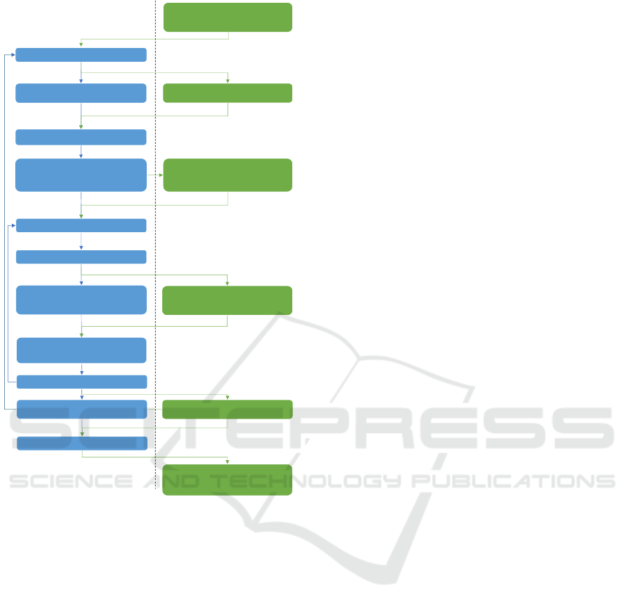
The ﬁgure 2 summarizes the modiﬁcations made

to the IDA algorithm for using the SPM.

3.4 Interface with Our Customized

Framework based on Modelica

OpenModelica (Fritzson et al., 2006) is an open-

source suite based on Modelica language (Fritzson

and Engelson, 1998), which is used for the modeling

and simulation of complex systems. It is an object-

oriented, formal and non-causal language for wri-

ting models in an equation-based style. Furthermore,

OpenModelica contains a compiler which enables to

generate simulation ﬁles, that are compatible with

IDA, from a Modelica model ﬁle. In particular, Mo-

delica enables to clearly separate the modeling and

solving aspects. The European projects PEGASE

(Chieh et al., 2011) and then iTesla (Vanfretti et al.,

2016) have introduced and proved the industrial po-

tential of Modelica for time-domain simulations of

transmission grids. Furthermore, the latter resulted in

the development of the iPSL library, which is open-

source and still maintained. Then, the dynamical-

study tools team of RTE implemented Dynamo, a new

simulation engine (Guironnet et al., 2018) which is

based on this framework. It especially enables to ea-

sily connect models with solvers to perform simulati-

ons in a very ﬂexible way.

Hence, in our framework, Modelica is used for the

modeling part of the simulation. Then, our objective

is to implement the model of the simulated system

SIMULTECH 2018 - 8th International Conference on Simulation and Modeling Methodologies, Technologies and Applications

Prediction: !

#$%

Correction residual evaluation &'!

#$%

(

Fourier coefficients update :

#$%

* +,

#$%

(

Fourier coefficients loading : ')

* +,

(

+ Continuity Condition: -

#./

Time step acceptability loop

Correction Jacobian evaluation

#$%

( + KLU factorization

Newton iterations loop

Newton linear system solving

Correction application : !

#$%

and !

#$%

Correction residual re-evaluation

&'!

#$%

(

Newton convergence test

Error test on !

#$%

Step size update

Prediction: -

#$%

+ Deduction of !

#$%

+ 3

5 and 3

5 evaluation

(for the estimator)

Correction application: -

#$%

and -

#$%

+ Deduction of !

#$%

and !

#$%

Error test on -

#$%

Figure 2: Modiﬁcation of the general algorithm of IDA

for integrating the SPM: the left part corresponds to the

standard IDA algorithm and the right part details the SPM-

speciﬁc operations.

with the Modelica language and, then, to perform the

simulation with IDASPM from Dynamo. To summa-

rize, in OpenModelica-type frameworks the simula-

tion process consists in three main steps:

1. The user implements a model from existing or

user-deﬁned libraries. A model generally consists

in assembling unit models within a global model

from their physical connections.

2. The model compiler, e.g. OpenModelica Compi-

ler, interprets this model to construct the associ-

ated DAE system to be solved. So, it constructs

a ”ﬂat model” by injecting all the mathematical

equations associated to the different unit com-

ponents and connections. In output of this pro-

cess, OpenModelica Compiler generates several

source ﬁles corresponding to the simulation: re-

sidual function of the DAE system, parameters,

initial values, etc.

3. To ﬁnish, as we have the ﬁles containing the

DAE system at our disposal, it can be integrated

using the chosen solver, e.g. SUNDIALS IDA.

To do this, our simulation engine contains generic

modules which automatically initialize the solver

data structures and data, and perform the simula-

tion from the chosen solver library.

Therefore, in order to interface our solver with

Dynamo, we have to generate the solver library cor-

responding to IDASPM and then to implement a cu-

stomized solver module which properly initializes

the data structures of IDASPM. In particular, it sup-

plies to IDASPM the pulsation of the system and the

boolean vector distinguishing the oscillating and non-

oscillating variables from a conﬁguration ﬁle. In the

current version of our implementation, this ﬁle is ma-

nually completed by the user and provided at execu-

tion time, which could be automatically done from

the modeler in a future version. Then, from these

data, IDASPM can be used for the simulation. Our

implementation does not require the initial Fourier

coefﬁcients to be set during the initialization. They

are computed directly during the simulation. This is

why performances are generally lower during the ﬁrst

time steps, even if the system is in steady-state. In-

deed some iterations are required for the Fourier coef-

ﬁcients to converge and consequently for the step size

to increase.

4 RESULTS AND DISCUSSION

4.1 Results on a Small Power System

First of all, our implementation has been tested on

a small three-phase power system with 4 nodes (see

ﬁgure 3). It contains 3 perfect generators, 1 resis-

tive load and connections with transmission lines mo-

deled with RL branches. In our framework, this mo-

del results in a system of 188 equations including

15 differential equations. Then, this system is sub-

ject to an exponential increase of the electrical load

at time t

event

= 1s. Our results have been obtained

from a Fedora Virtual Machine (launched from Vir-

tualBox) running with 2 processors (CPU: Intel i5-

5257U @2.7GHz, cache=3MB) and 4GB of RAM.

The ﬁgure 4 shows that the solution obtained with

IDASPM perfectly ﬁts with those obtained with IDA.

Then, in the ﬁgure 5, the step sizes used by IDA and

IDASPM are compared. Then, we can see that the

SPM globally enables to integrate the DAE with much

larger time steps. As expected, the step size used with

Use of the Sinusoidal Predictor Method within a Fully Separated Modeler/Solver Framework for Fast and Flexible EMT Simulations

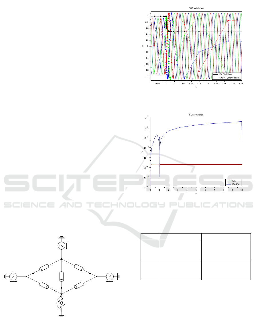
the SPM reaches high values when the system is in

steady-state. Hence, one can identify three time inter-

vals:

1. From the beginning of the simulation to the event,

the step size increases regularly. At the very be-

ginning, the SPM uses small time steps as the

Fourier coefﬁcients are initialized to zero. Then,

some iterations are required for them to converge.

2. During the load variation, the step size remains

at very low values. As the estimator is designed

from the assumption that the system is in steady-

state, this step size limitation is logical.

3. When the system returns to steady-state, the step

size increases again and reaches high values.

Hence, IDASPM requires 157 time steps and 0.64

seconds to perform the simulation. IDA requires

52115 time steps and 2.69 seconds to perform the si-

mulation. Their performances are summarized in ta-

ble 1. So, using the SPM enables to dramatically re-

duce the number of iterations for performing this si-

mulation (divided by more than 300). The speedup

is also signiﬁcant (divided by 4). However, we can

see that it is not as important as for the number of ite-

rations. Indeed, the SPM requires to perform more

mathematical operations whose computational cost is

not negligible than a classical integration method. In

particular, as our current implementation is not com-

pletely optimized, the computational cost of the esti-

mator remains important. This cost is mainly due to

the use of the Jacobian matrix of the DAE system and

the different linear algebra operations that are done

during the estimation process. This is why the ﬁnal

computational time by iteration is currently high.

Figure 3: Simple Electrical Grid test case (ﬁgure from (Gi-

bert et al., 2018)).

Figure 4: Comparison of the solutions obtained with IDA

(full line) and IDASPM (dashed line) on the Simple Elec-

trical Grid test case (tolerance = 1.e-4).

Figure 5: Comparison on the step size used by IDA (red

line) and IDASPM (blue line) on the Simple Electrical Grid

test case with tol=1.e-4.

Table 1: Performances comparison between IDA and

IDASPM on the SEG test case.

tol Method SEG

IDA 52115 it. (2.69 s)

1.e-4 IDASPM 157 it. (0.64 s)

IDA/IDASPM 332 (4.20)

IDA 112035 it. (6.65 s)

1.e-5 IDASPM 290 it. (0.76 s)

IDA/IDASPM 386 (8.75)

4.2 Results on a Customized Version of

the IEEE 14-bus Reference Test

Case

Then, our implementation has been tested on a larger

power system with 14 nodes (see ﬁgure 6), inspired

on the reference test case IEEE-14 bus. Its contains

5 perfect generators, 11 resistive loads, connections

with transmission lines modeled with RL branches

and ideal transformers. In our framework, this mo-

del results in a system of 754 equations including 51

SIMULTECH 2018 - 8th International Conference on Simulation and Modeling Methodologies, Technologies and Applications

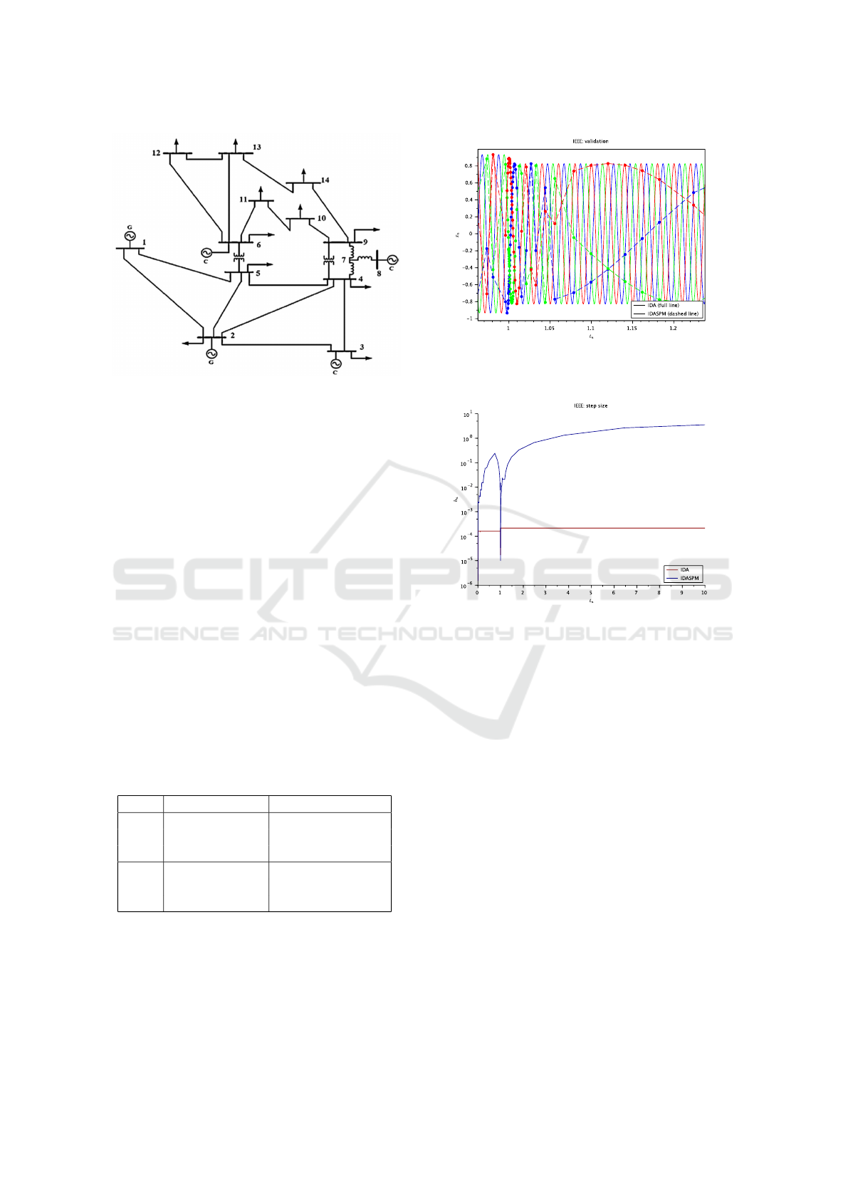
Figure 6: IEEE 14-bus test case (ﬁgure from (Abbas Taher

et al., 2015)).

differential equations. Then, this system is subject to

an exponential increase of the electrical load attached

to Bus 4 at time t

event

= 1s.

The ﬁgure 7 shows that the solution obtained with

IDASPM perfectly ﬁts with those obtained with IDA.

In ﬁgure 8, the step sizes used by IDA and IDASPM

are compared. Results are very similar to those obtai-

ned on the Simple Electrical Grid test case. Indeed,

IDASPM requires 174 time steps and 11.66 seconds

to perform the simulation. IDA requires 48504 time

steps and 3.21 seconds to perform the simulation.

Their performances are summarized in table 2. Then,

as for the Simple Electrical Grid test case, the num-

ber of time steps is very signiﬁcantly reduced by using

the SPM. However, as the computational cost by ite-

ration is still too important in our current version of

IDASPM, there is ﬁnally no speedup. Further deve-

lopments will focus on optimizing the Fourier coefﬁ-

cients estimator, which represents the large majority

of the computational time.

Table 2: Performances comparison between IDA and

IDASPM on the IEEE 14-bus inspired test case.

tol Method IEEE-14

IDA 48504 it. (3.21 s)

1.e-4 IDASPM 174 it. (11.66 s)

IDA/IDASPM 279 (0.28)

IDA 116705 it. (7.90 s)

1.e-5 IDASPM 306 it. (13.24 s)

IDA/IDASPM 381 (0.60)

4.3 Discussion and Area for

Improvement of IDASPM

In conclusion, in spite of the large reduction of num-

ber of iterations for performing time-domain simula-

tions, the ﬁnal speedup with our current implementa-

Figure 7: Comparison of the solutions obtained with IDA

(full line) and IDASPM (dashed line) on the IEEE 14-bus

inspired test case (tolerance = 1.e-4).

Figure 8: Comparison on the step size used by IDA (red

line) and IDASPM (blue line) on the IEEE 14-bus inspired

test case (tolerance = 1.e-4).

tion of IDASPM is low for some test cases. For in-

stance, on the IEEE 14-bus inspired test case, using

IDASPM leads to a greater computational time while

the number of iterations is divided by a factor close

to 300. On the contrary, on the SEG test case, the

speedup is signiﬁcant but still could be enhanced.

If we consider the computational time by iteration,

we can see that it is

• for SEG, 4.1ms/it. with tol.=1.e-4 and 2.6ms/it.

with tol.=1.e-5;

• for IEEE, 67ms/it. with tol.=1.e-4 and 43ms/it.

with tol.=1.e-5.

In other words, the computational time by itera-

tion is about 16 times greater between SEG and IEEE,

i.e. the dimension increase factor squared. So, we can

see that our implementation is currently very sensitive

to the problem dimension. One can note that the com-

putational time is lower when reducing the tolerance

on average. This is due to the IDA management of

Jacobian updates. Indeed, while the number of ite-

rations is almost twice when passing from tol=1.e-4

Use of the Sinusoidal Predictor Method within a Fully Separated Modeler/Solver Framework for Fast and Flexible EMT Simulations

to tol=1.e-5, there are only 2 additional Jacobian up-

dates. Then, we used KCacheGrind (Weidendorfer,

2008) to proﬁle the performances of our implemen-

tation. Two functions cover the large majority of the

solving process:

1. The linear solver setup function, which performs

the Jacobian evaluation and factorization. The se-

tup function represents 24.64% of the global com-

putational cost. In particular, the relative cost

of the Jacobian evaluation is 23.02%, i.e. about

93.43% of the setup.

2. The Fourier coefﬁcient update function represents

75.29% of the global computational cost. In parti-

cular the relative cost of the matrix factorization,

that is done for solving the linear system of the

estimator (16), is 67.20%, i.e. 89.25% of the esti-

mator cost.

Therefore, these ﬁrst investigations make several

optimization ideas evident:

• In IDA, the Jacobian matrix of the DAE system is

given by the formula (9) i.e. J

= ∂

F + c

∂

Then, as our Fourier coefﬁcients estimator requi-

res the two partial derivatives of F, ∂

F and ∂

the current implementation of IDASPM calls the

Jacobian matrix evaluation function three times:

once for evaluating the solver full Jacobian which

is used for the integration process (with the c

coefﬁcient of the integrator) and twice for eva-

luating the two partial derivatives (with c

= 0

for the X partial derivative and with c

= −1 for

preparing the

X partial derivative extraction). In

addition, each Jacobian matrix evaluation calls a

modeler-level function which computes the Jaco-

bian matrix by performing an automatic differen-

tiation of the residual function. To ﬁnish, once the

Jacobian matrix evaluations have been done for

the estimator, some matrix operations are requi-

red for extracting the

X partial derivative. So, our

ﬁrst optimization idea consists in modifying the

IDASPM Jacobian evaluation function for ﬁlling

the three different Jacobian matrix in a single call.

Indeed, in the modeler-level code, the two partial

derivatives are evaluated and then added. By this

way, an important computational time could be

saved.

• Furthermore, the current implementation ﬁlls a

dense matrix for the estimator linear system from

the sparse Jacobian matrix of the system. Howe-

ver, as the estimator matrix should also be very

sparse, an important computational time could be

saved by solving this linear system with the KLU,

which is a sparse solver.

• In addition, we noted that there are signiﬁcantly

more Jacobian updates when using IDASPM

compared with IDA. Generally, the Jacobian ma-

trix is updated by the integrator when the Newton

algorithm fails to converge. These convergence

fails may be due to major changes in Jacobian ma-

trix. However, there is no apparent reason for the

Jacobian matrix of IDASPM to change more than

those of IDA. This point is to investigate, espe-

cially as updating the Jacobian matrix requires to

perform a new factorization for the Newton itera-

tions.

• To ﬁnish, in our current implementation of

IDASPM within Dynamo, the Fourier coefﬁcients

are set to zero. Then, for each tested case, we can

see that the step size is limited at the very begin-

ning of the simulation. So, by properly initializing

the Fourier coefﬁcients, some iterations could be

saved at that very time. However, the presented

results prove the robustness of the estimator as

Fourier coefﬁcients converge in a few number of

iterations.

5 CONCLUSIONS

In conclusion, the implementation presented in this

paper paves the way to long-term EMT simulations

of power systems within a very ﬂexible framework.

Using Modelica and especially our customized envi-

ronment based on OpenModelica enables to clearly

distinguish the modeling and solving aspects of the si-

mulation. Furthermore, using the proposed IDASPM

solver leads to a very important reduction of the num-

ber of iterations for performing a simulation, com-

pared to the original IDA solver. However, as the

current implementation of our method is not comple-

tely optimized, there is no speedup on larger test ca-

ses. Therefore, our further developments will focus

on optimizing the estimator, in which the main part of

the computational time is currently spent. Indeed, as

mentioned in the results discussion, some accessible

enhancements are envisioned, especially for reducing

the computational cost of linear algebra operations. In

addition, we could investigate strategies for activating

and deactivating the Fourier coefﬁcients update du-

ring transient phases. Indeed, in such phases, as the

Fourier estimation is perturbed, the step size is ﬁnally

limited.

SIMULTECH 2018 - 8th International Conference on Simulation and Modeling Methodologies, Technologies and Applications

ACKNOWLEDGMENT

The authors would like to thank the French Natio-

nal Research Agency in Technology who founded this

project under the contract CIFRE n

2015/0885.

REFERENCES

Abbas Taher, S., Mahmoodi, H., and Aghaamouei, H.

(2015). Optimal pmu location in power systems using

mica. Alexandria Engineering Journal.

Astic, J., Bihain, A., and Jerosolimski, M. (1994). The

mixed adams-bdf variable step size algorithm to si-

mulate transient and long term phenomena in po-

wer systems. IEEE Transactions on Power Systems,

9(2):929–935.

Brayton, R. K., Gustavson, F. G., and Hachtel, G. D. (1972).

A new efﬁcient algorithm for solving differential-

algebraic systems using implicit backward differenti-

ation formulas. Proceedings of the IEEE, 60(1):98–

108.

Chieh, A. S., Panciatici, P., and Picard, J. (2011). Power

system modeling in modelica for time-domain simu-

lation. In PowerTech, 2011 IEEE Trondheim, pages

1–8. IEEE.

CRSA, RTE, TE, and TU/e (2011). D4.1: Algorithmic re-

quirements for simulation of large network extreme

scenarios. Technical report, PEGASE Consortium.

Demiray, T. (2008). Simulation of power system dynamics

using dynamic phasor models. PhD thesis, ETH Zu-

rich.

Demiray, T., Milano, F., and Andersson, G. (2007). Dyna-

mic phasor modeling of the doubly-fed induction ge-

nerator under unbalanced conditions. In Power Tech,

2007 IEEE Lausanne, pages 1049–1054. IEEE.

Fritzson, P., Aronsson, P., Pop, A., Lundvall, H., Ny-

strom, K., Saldamli, L., Broman, D., and Sandholm,

A. (2006). Openmodelica: A free open-source en-

vironment for system modeling, simulation, and te-

aching. In Computer Aided Control System Design,

2006 IEEE International Conference on Control Ap-

plications, 2006 IEEE International Symposium on

Intelligent Control, 2006 IEEE, pages 1588–1595.

IEEE.

Fritzson, P. and Engelson, V. (1998). Modelica: A uni-

ﬁed object-oriented language for system modeling

and simulation. In European Conference on Object-

Oriented Programming, pages 67–90. Springer.

Gibert, P.-M., Losseau, R., Guironnet, A., Panciatici, P.,

Tromeur-Dervout, D., and Erhel, J. (2018). Speedup

of emt simulations by using an integration scheme en-

riched with a predictive fourier coefﬁcients estimator.

under review.

Gibert, P.-M., Tromeur-Dervout, D., Panciatici, P., Beaude,

F., Wang, P., and Erhel, J. (2017). A generic cu-

stomized predictor corrector approach for accelera-

ting emtp-like simulations. In PowerTech, 2017 IEEE

Manchester, pages 1–6. IEEE.

Guironnet, A., Saugier, M., Petitrenaud, S., Xavier, F., and

Panciatici, P. (2018). Towards an open-source solution

using modelica for time-domain simulation of power

systems. under review.

Hindmarsh, A. C., Brown, P. N., Grant, K. E., Lee, S. L.,

Serban, R., Shumaker, D. E., and Woodward, C. S.

(2005). Sundials: Suite of nonlinear and differen-

tial/algebraic equation solvers. ACM Transactions on

Mathematical Software (TOMS), 31(3):363–396.

Petzold, L. R. et al. (1982). A description of dassl: A diffe-

rential/algebraic system solver. Scientiﬁc computing,

1:65–68.

Scilab, E. et al. (2012). Scilab: Free and open source soft-

ware for numerical computation. Scilab Enterprises,

Orsay, France, page 3.

Vanfretti, L., Rabuzin, T., Baudette, M., and Murad, M.

(2016). itesla power systems library (ipsl): A mo-

delica library for phasor time-domain simulations.

SoftwareX, 5:84–88.

Weidendorfer, J. (2008). Sequential performance analysis

with callgrind and kcachegrind. In Tools for High Per-

formance Computing, pages 93–113. Springer.

Use of the Sinusoidal Predictor Method within a Fully Separated Modeler/Solver Framework for Fast and Flexible EMT Simulations