
Numerical Investigation of Newton’s Method for Solving Discrete-time
Algebraic Riccati Equations
Vasile Sima
1
and Peter Benner
2
1
Modelling, Simulation, Optimization Department, National Institute for Research & Development in Informatics,
Bd. Mares¸al Averescu, Nr. 8–10, Bucharest, Romania
2
Max Planck Institute for Dynamics of Complex Technical Systems, Sandtorstraße 1, Magdeburg, Germany
Keywords:
Algebraic Riccati Equation, Numerical Methods, Optimal Control, Optimal Estimation.
Abstract:
A Newton-like algorithm and some line search strategies for solving discrete-time algebraic Riccati equations
are discussed. Algorithmic and implementation details incorporated in the developed solver are described.
Some numerical results of an extensive performance investigation on a large collection of examples are sum-
marized. These results often show significantly improved accuracy, measured in terms of normalized and
relative residuals, in comparison with the state-of-the-art MATLAB function. The new solver is strongly
recommended for improving the solutions computed by other solvers.
1 INTRODUCTION
Many procedures for control systems analysis and de-
sign require the solution of algebraic Riccati equa-
tions (AREs). Such equations appear in various do-
mains and practical applications, including model re-
duction, optimal filtering, guidance, (robust) control,
robotics, etc. Discrete-time AREs (DAREs) are im-
portant since many measured systems are modeled by
difference equations. Let A, E ∈ R
n×n
, B ∈ R
n×m
,
and Q and R be symmetric matrices of suitable dimen-
sions. In a compact notation, the generalized DAREs,
with unknown X = X
T
∈ R
n×n
, are defined by
0 = Q+ op(A)
T
X op(A) − op(E)
T
X op(E)
−σL(X)
ˆ
R(X)
−1
L(X)
T
=: R (X), (1)
where σ = ±1, E and
ˆ
R(X) are nonsingular, and
ˆ
R(X) := R+ σB
T
XB,
L(X) := S+ op(A)
T
XB, (2)
with S of suitable size. The operator op(M) repre-
sents either M or M
T
, corresponding to a control or a
filtering problem, respectively. A and E are the state
and descriptor matrices, respectively, of a linear time-
invariant dynamic system, and, in a control setting, B
is the input matrix. The use of the ± sign through σ
offers a greater generality. In practice, often Q and
S are expressed as C
T
ˆ
QC and S = C
T
ˆ
S, respectively,
where C ∈ R
p×n
is the output matrix of the system,
and C,
ˆ
Q, and
ˆ
S are given.
The solutions of a DARE are the matrices X = X
T
for which R (X) = 0. Usually, what is needed is
a stabilizing solution, X
s
, for which the matrix pair
(A − σop(BK(X
s
)),E) is stable (in a discrete-time
sense), where op(K(X
s
)) is the gain matrix of the op-
timal regulator or estimator, given by
K(X) :=
ˆ
R(X)
−1
L(X)
T
, (3)
with X replaced by X
s
. For the dynamic system
Ex
k+1
= Ax
k
+ Bu
k
, k = 0, 1,..., x(0) = x
0
, the op-
timal control trajectory is given by the state feedback
law u
k
= −σK(X
s
)x
k
. By a proper selection of Q, S,
and R, the closed-loop dynamics can be modified to
achieve a fast transient response, disturbance rejec-
tion, etc. Note that for a filtering problem, B should
be replaced by the transpose of C, and the computed
K(X) is the transpose of the filter gain matrix. When
Y is not a solution of (1), then R (Y) differs from the
zero matrix; R (Y) is called the residual of (1) in Y.
The Frobenius norm of R (Y), kR (Y)k
F
, is a measure
of the error in Y with respect to the solution X.
There is an impressive literature concerning the-
ory and numerical solution of AREs and their practi-
cal applications. Several monographs, e.g., (Ander-
son and Moore, 1971; Bini et al., 2012; Lancaster
and Rodman, 1995; Mehrmann, 1991; Sima, 1996)
address various theoretical and practical results. Ex-
istence and uniqueness results for ARE solutions are
dealt with, for instance, in (Lancaster and Rodman,
1980; Lancaster et al., 1986; Lancaster et al., 1987).
66
Sima, V. and Benner, P.
Numerical Investigation of Newton’s Method for Solving Discrete-time Algebraic Riccati Equations.
DOI: 10.5220/0006860600660075
In Proceedings of the 15th International Conference on Informatics in Control, Automation and Robotics (ICINCO 2018) - Volume 1, pages 66-75
ISBN: 978-989-758-321-6
Copyright © 2018 by SCITEPRESS – Science and Technology Publications, Lda. All rights reserved

Many “direct” or iterative algorithms have been pro-
posed for solving AREs. The first class includes
the (generalized) Schur techniques, e.g., (Arnold and
Laub, 1984; Kenney et al., 1989; Laub, 1979; Pap-
pas et al., 1980; Van Dooren, 1981), or structure-
exploiting (QR-like) methods, e.g., (Bunse-Gerstner
and Mehrmann, 1986; Sima and Benner, 2015; Ben-
ner et al., 2016). (These techniques are actually also
iterative, but they are applied to a matrix or matrix
pencil defined by the given matrices of an ARE.) The
second class has several categories, including sign
function techniques, e.g., (Balzer, 1980; Byers, 1987;
Gardiner and Laub, 1986; Roberts, 1980; Sima and
Benner, 2008), Newton techniques, e.g., (Anderson,
1978; Arnold and Laub, 1984; Guo and Laub, 2000;
Hammarling, 1982), doubling algorithms, e.g., (Chu
et al., 2005; Guo et al., 2006; Guo et al., 2007; Guo,
2016), or recursive algorithms (Lanzon et al., 2008).
Newton’s method for solving AREs has been
considered by many authors, for instance, (Klein-
man, 1968; Hewer, 1971; Arnold and Laub, 1984;
Mehrmann, 1991; Lancaster and Rodman, 1995;
Sima, 1996; Benner, 1997; Benner, 1998; Benner
and Byers, 1998). Moreover, the matrix sign func-
tion method for AREs, see (Byers, 1987; Gardiner
and Laub, 1986) and the references therein, is actu-
ally a specialization of Newton’s method for comput-
ing the square root of the identity matrix of order 2n.
Newton’s method is best used for iterative im-
provement of a solution, or as a defect correction
method (Mehrmann and Tan, 1988), delivering the
maximal possible accuracy when starting from a good
approximate solution. Moreover, it may be preferred
in implementing certain fault-tolerant or slowly vary-
ing systems, which require online controller updat-
ing (Ciubotaru and Staroswiecki, 2009); then, the pre-
viously computed ARE solution can be used for ini-
tialization. Some robotics applications can also ben-
efit from using iterative ARE solvers. For this rea-
son, such algorithms are used in a new open-source
C++ library for robotics, optimal and model predic-
tive control (Giftthaler et al., 2018), for solving both
continuous-time AREs (CAREs) and DAREs.
This paper summarizes the main theoretical facts
about Newton’s method for DAREs, as well as imple-
mentation issues and numerical results obtained using
the newly developed solver. There are several contri-
butions comparing to (Benner, 1998; Benner and By-
ers, 1998) concerning, e.g., generality and function-
ality, line search strategies, or stopping criteria. The
paper complements our previous studies on the nu-
merical solution of CAREs by Newton’s method with
line search reported in (Sima and Benner, 2014; Sima,
2015).
2 CONCEPTUAL ALGORITHM
The following Assumptions are made:
1. Matrix E is nonsingular.
2. Matrix pair ( op(E)
−1
op(A), op(E)
−1
B) is stabi-
lizable.
3. Matrix R = R
T
is non-negative definite (R ≥0).
4. A stabilizing solution X
s
exists and it is unique,
and
ˆ
R(X
s
) is positive definite (
ˆ
R(X
s
) > 0).
Note that Assumption 1 is not actually used by the
developed solver, contrary to other solvers (including
MATLAB function
dare
).
The algorithmic variants considered in the se-
quel for DAREs are extensions of Newton’s method,
which employ a line search procedure attempting to
reduce the residual along the Newton direction.
The conceptual algorithm can be stated as fol-
lows (Benner, 1998):
Algorithm NDARE: Modified Newton method for
DARE
Input: The coefficient matrices E, A, B, Q, R, and S,
and an initial matrix X
0
= X
T
0
.
Output: The approximate solution X
k
of DARE (1).
FOR k = 0, 1, ...,k
max
, DO
1. Compute R (X
k
). If convergence or non-
convergence is detected, return X
k
and/or a warn-
ing or error indicator value.
2. Compute K
k
:= K(X
k
) in (3) and op(A
k
), where
A
k
= op(A) −σBK
k
.
3. Solve the discrete-time generalized Stein equation
op(A
k
)
T
N
k
op(A
k
) −op(E)
T
N
k
op(E) = −R (X
k
)
(4)
for N
k
.
4. Find a step size t
k
which approximatelyminimizes
kR (X
k
+ tN
k
)k
2
F
, with respect to t.
5. Update X
k+1
= X
k
+ t
k
N
k
.
END
Equation (4) is also called discrete-time generalized
Lyapunov equation. The usual, standard Lyapunov
equation has E = I
n
.
Standard Newton algorithm is obtained by taking
t
k
= 1 in Step 4 at each iteration. When the initial ma-
trix X
0
is far from a Riccati equation solution, New-
ton’s method with line search often outperforms the
standard Newton’s method.
If the assumptions above hold and X
0
is stabiliz-
ing, then the iterates of the Algorithm NDARE with
σ = 1 and t
k
= 1 have the following properties (Ben-
ner, 1997):
(a) All matrices X
k
are stabilizing.
Numerical Investigation of Newton’s Method for Solving Discrete-time Algebraic Riccati Equations
67

(b) X
s
≤ ··· ≤ X
k+1
≤ X
k
≤ ··· ≤ X
1
.
(c) lim
k→∞
X
k
= X
s
.
(d) There is a constant γ > 0 such that
kX
k+1
−X
s
k ≤ γk X
k
−X
s
k
2
, k ≥1. (5)
Note that the global quadratic convergence for-
mula (5) does not hold for k = 0, involving the iterates
X
0
and X
1
.
Weaker results are available for the modified New-
ton algorithm. One such result (Benner, 1997) states
that if X
k
is stabilizing, then N
k
computed by Algo-
rithm NDARE is a descent direction for kR (X
k
)k
2
F
from X
k
, unless X
k
= X
s
.
3 ALGORITHMIC DETAILS
Algorithm NDARE was implemented in a For-
tran 77 subroutine,
SG02CD
, following the SLICOT
Library (Benner et al., 1999; Benner and Sima,
2003; Benner et al., 2010; Van Huffel et al., 2004)
implementation and documentation standards (see
http://www.slicot.org). The same routine also solves
CAREs. A first version of
SG02CD
and preliminary
results on random examples and SLICOT CAREX
benchmark collection (Abels and Benner, 1999a)
have been presented in (Sima and Benner, 2006). The
implemented solver deals with generalized DAREs
without inverting the matrix E, which is very im-
portant for numerical reasons, since E might be
ill-conditioned with respect to inversion. Standard
DAREs are solved with the maximal possible effi-
ciency. Moreover, both control and filter DAREs
can be solved by the same routine, using an option
(“mode”) parameter, which specifies the op operator.
The matrices A and E are not transposed.
The essential computational procedures involved
in Algorithm NDARE are detailed below.
3.1 Removing S Matrix
If R is nonsingular, DAREs can be put in a simpler
form, which is more convenient for Newton algo-
rithms. Specifically, setting
˜
A = A−σop(BR
−1
S
T
),
˜
Q = Q−σSR
−1
S
T
, (6)
after redefining A and Q as
˜
A and
˜
Q, respectively,
equation (1) reduces to
0 = op(A)
T
X op(A) − op(E)
T
X op(E)
−σop(A)
T
X
ˆ
G(X)X op(A) + Q =: R (X),(7)
where
ˆ
G(X) := B
ˆ
R(X)
−1
B
T
, and the second term re-
duces to X in the standard case (E = I
n
). The trans-
formations in (6) eliminate the matrix S from the for-
mulas to be used. In this case, the matrix K
k
may
sometimes no longer be computed in Step 2, and
A
k
= op(A) −σ
ˆ
G
k
X
k
op(A), with
ˆ
G
k
:=
ˆ
G(X
k
).
To obtain
˜
A and
˜
Q in (6), the Cholesky factor of
R, R
c
, can be used if R > 0, where R =: R
T
c
R
c
, with R
c
upper triangular. Defining
˜
B = BR
−1
c
and
˜
S = SR
−1
c
,
the relations (6) are equivalent to
˜
A = A−σop(
˜
B
˜
S
T
),
˜
Q = Q−σ
˜
S
˜
S
T
, (8)
so just two triangular systems need to be solved,
and two matrix products are computed for obtaining
˜
A and
˜
Q, after factoring R. Symmetry is exploited
for getting
˜
Q via a BLAS (Dongarra et al., 1990)
symm operation. Similarly, if
ˆ
R(X
k
) > 0, then the
Cholesky factor of
ˆ
R(X
k
),
ˆ
R
c
(X
k
), can be used. Defin-
ing D
k
:= D(X
k
) := B
ˆ
R
c
(X
k
)
−1
, then
ˆ
G
k
= D
k
D
T
k
, and
A
k
= op(A) −σD
k
D
T
k
X
k
op(A). The use of D
k
instead
of
ˆ
G
k
is convenient when m is sufficiently smaller
than n (m ≤ n/4). If
ˆ
G
k
is to be preferred (since
m > n/4), but the norm of
ˆ
G
0
is too large, then, if
possible, the factor D
k
is used in the iterative process
instead of
ˆ
G
k
, in order to potentially improve the nu-
merical behavior, even if the efficiency somewhat di-
minishes.
When R is not positive definite, then either UDU
T
or LDL
T
factorization (Golub and Van Loan, 1996) of
R can be employed for computing
˜
A and
˜
Q. Similarly,
UDU
T
/LDL
T
factorization of
ˆ
R(X
k
) can be used for
obtaining
ˆ
G
k
, when
ˆ
R(X
k
) is indefinite.
3.2 Using S Matrix
When S 6= 0, but R is ill-conditioned with respect to
inversion, the use of formulas (6) will potentially in-
troduce large errors from the beginningof the iterative
process, which will be propagated during the entire
process. This might involve a degradation of its be-
havior, resulting in slower convergence, and/or an in-
accurate computed solution. Using S during the itera-
tive process could avoid such degradation. Therefore,
an option of the solver allows to avoid the transforma-
tions (6), and involve S in all subsequent calculations.
In this case, other formulas are needed, since
ˆ
G
k
can-
not be used. Specifically, define
H
k
:= op(A
k
)
T
X
k
B+ S, F
k
= H
k
ˆ
R
c
(X
k
)
−1
, (9)
with
ˆ
R
c
(X
k
) introduced above; for having F
k
it is as-
sumed here that
ˆ
R(X
k
) > 0. (H
k
is a convenient no-
tation for L(X
k
).) Then, the residual R (X
k
) and the
matrix A
k
can be computed using
R (X
k
) = Q+ op(A)
T
X
k
op(A)
−op(E)
T
X
k
op(E) −σF
k
F
T
k
, (10)
A
k
= op(A) −σD
k
F
T
k
, (11)
where D
k
has been defined above.
ICINCO 2018 - 15th International Conference on Informatics in Control, Automation and Robotics
68

If, however,
ˆ
R(X
k
) is indefinite, then the needed
formulas follow directly from (1)–(3), namely,
R (X
k
) = Q+ op(A)
T
X
k
op(A)
−op(E)
T
X
k
op(E) −σH
k
K
k
, (12)
A
k
= op(A) −σBK
k
, (13)
involving the UDU
T
or LDL
T
factorization of
ˆ
R(X
k
).
Moreover, symmetry of the matrix product H
k
K
k
is
taken into account. (The solver computes either the
upper or lower triangle of R (X
k
).)
The implementation is optimized by using com-
mon subexpressions when computing R (X
k
) and
op(A
k
), taking also into account the ratio between n
and m. Various formulas for efficient implementation
of Newton’s method for AREs are proven in (Sima,
2014).
3.3 Initialization and Main Options
The iteration is started by an initial (stabilizing) ma-
trix X
0
, which may not be given on input, if the zero
matrix can be used. If X
0
is not stabilizing, and find-
ing X
s
is not required, Algorithm NDARE could con-
verge to another DARE solution.
Since the solution computed by a Newton algo-
rithm generally depends on initialization, another op-
tion specifies if the stabilizing solution X
s
is to be
found. This is assumed to be the case in the sequel.
The initial matrix X
0
must then be stabilizing, and a
warning is issued if this property does not hold; more-
over, if the computed X is not stabilizing, an error is
issued.
Another option specifies whether to use standard
Newton’s method, or one of the modified Newton’s
method variations, discussed in a paragraph below,
which employ a line search strategy.
Optionally, the matrices A
k
and E (if E is gen-
eral) are scaled for solving the Stein equations, and
their solutions are suitably updated. Note that the
LAPACK subroutines
DGEES
and
DGGES
(Anderson
et al., 1999), which are called by the standard and
generalized Stein solvers, respectively, to compute the
real Schur(-triangular) form, do not scale the coeffi-
cient matrices. Just column and row permutations are
performed, to separate isolated eigenvalues. For some
examples, and no scaling, the convergence was not
achieved in a reasonable number of iterations. More-
over, sometimes scaling allows to compute more ac-
curate solutions and/or use less iterations, comparing
to the case with no scaling.
A maximum allowed number of iteration steps,
k
max
, is specified on input, and the number of itera-
tion steps performed, k
s
, is returned on exit.
3.4 Finding the Step Size
The optimal step size t
k
is given by
t
k
= argmin
t
kR (X
k
+ tN
k
)k
2
F
. (14)
Since solving (14) for a DARE is expensive, it was
suggested in (Benner, 1997; Benner, 1998) to use an
approximate value t
k
to be found numerically as the
argument of the minimal value in [0,2] of a polyno-
mial of order 4. Indeed,
R (X
k
+ tN
k
) = (1 −t)R (X
k
) −t
2
V
k
, (15)
where V
k
= op(A
k
)
T
N
k
ˆ
G
k
N
k
op(A
k
). The prob-
lem (14) is replaced by the minimization of the ap-
proximate quartic polynomial (Benner, 1997)
f
k
(t) := trace(R (X
k
+ tN
k
)
2
)
≈ α
k
(1−t)
2
−2β
k
(1−t)t
2
+ γ
k
t
4
, (16)
where α
k
= trace(R (X
k
)
2
), β
k
= trace(R (X
k
)V
k
),
γ
k
= trace(V
2
k
).
To solve this problem, a cubic polynomial (the
derivative of f
k
(t)) is set up, whose roots in [0,2], if
any, are candidates for the solution of the approximate
minimum residual problem. The roots of this cubic
polynomial are computed by solving an equivalent 4-
by-4 standard or generalized eigenproblem, following
(J´onsson and Vavasis, 2004).
Actually, the true f
k
(t) for DAREs is a rational
function, and the above formulas are obtained by
replacing its denominator by the second order Tay-
lor series approximant at t = 0. The approximation
is useful when t is small enough. For instance, if
t < 1/k
ˆ
G
k
N
k
k, where k · k is any submultiplicative
norm, then
ˆ
R(X
k+1
) := R+ B
T
(X
k
+t
k
N
k
)B is nonsin-
gular, if
ˆ
R(X
k
) is nonsingular. Since t
k
is chosen from
the interval [0,2], the condition above is satisfied if
k
ˆ
G
k
N
k
k< 1/2. It can be shown (Benner, 1997) that if
X
k
is stabilizing, then either N
k
is a descent direction
for kR (X
k
)k
2
F
, or X
k
= X
s
. But the stabilizing prop-
erty is not guaranteed, at least for t ∈ [0,2]. When
k
ˆ
G
k
N
k
k is large (usually, at the beginning of the iter-
ative Newton process), the step sizes t
k
could be too
small, and the progress of the iteration could be too
slow.
3.5 Iterative Process
The algorithm computes the initial residual matrix
R (X
0
) and the matrix op(A
0
), where A
0
:= op(A) −
σ
ˆ
G
0
X
0
op(A). If no initial matrix X
0
is given, then
X
0
= 0, R (X
0
) =
˜
Q and op(A
0
) =
˜
A in (6).
At the beginning of the iteration k, 0 ≤ k ≤ k
max
,
the algorithm decides to terminate or continue the
Numerical Investigation of Newton’s Method for Solving Discrete-time Algebraic Riccati Equations
69

computations, based on the current normalized resid-
ual r
k
(and possible on relative residual r
r
(X
k
)), de-
fined below. If min(r
k
,r
r
(X
k
)) > τ, a standard (if
E = I
n
) or generalized Stein equation (4) is solved for
N
k
(the Newton direction).
The basic stopping criterion for the iterative pro-
cess is stated in terms of a normalized residual, r
k
:=
r(X
k
), and a tolerance τ. If
r
k
:= kR (X
k
)k
F
/max(1,kX
k
k
F
) ≤ τ, (17)
the iterative process is successfully terminated. If τ ≤
0, a default tolerance is used, defined in terms of the
Frobenius norms of the given matrices, and relative
machine precision, ε
M
. Specifically, τ is computed by
the formula
τ = min{ε
M
√
n
kAk
F
(kAk
F
+ kD
0
k
2
F
kAk
F
)
+ kEk
2
F
+ kQk
F
,
√
ε
M
/10
3
}. (18)
(The factor kD
0
k
2
F
is replaced by
ˆ
G
0
if
ˆ
R(X
0
) is indef-
inite.) The second operand of min in (18) was intro-
duced to prevent deciding convergence too early for
systems with very large norms for A, E, D
0
(or
ˆ
G
0
),
and/or Q.
For systems with very large norms of the ma-
trices A, E, D
0
(or
ˆ
G
0
), and/or Q, and small norm
of the solution X, the termination criterion involv-
ing (18) might not be satisfied in a reasonable num-
ber of iterations (or never, due to accumulated round-
ing errors), while an acceptable approximate solu-
tion might be much earlier available. Therefore, the
MATLAB-style relative residual, r
r
(X
k
), which in-
cludes the Frobenius norms of the four matrix terms
of (1) in the denominator of its formula, is also tested
at iterations 10 + 5q, q = 0,1,..., and it might pro-
duce the termination of the iterative process, instead
of the criterion based on the normalized residual. The
relative residual is not tested at each iteration in or-
der to reduce the computation costs, and to increase
the chances of termination via the normalized resid-
ual test.
Another test is to check if updating X
k
is meaning-
ful. The updating is done if t
k
kN
k
k
F
> ε
M
kX
k
k
F
. If
this is the case, set X
k+1
= X
k
+t
k
N
k
, and compute the
updated matrices op(A
k+1
) and R (X
k+1
). Otherwise,
the iterativeprocess is terminated and a warning value
is set, since no further significant, but only marginal
improvements can be expected, eventually after many
additional iterations. Although the computation of the
residual R (X
k
+t
k
N
k
) can be efficiently performed by
updating the residual R (X
k
), the original data is used,
since the updating formula (15) could suffer from se-
vere numerical cancellation, and hence it could com-
promise the accuracy of the intermediate results.
Often, but mainly in the first iterations, the com-
puted optimal steps t
k
are too small, and the resid-
ual decreases too slowly. This is called stagnation,
and remedies are used to escape stagnation, as de-
scribed below. The chosen strategy was to set t
k
= 1
when stagnation is detected, but also when t
k
< 0.5,
ε
1/4
M
< r
k
< 1, and kR (X
k
+t
k
N
k
)k
F
≤10, if this hap-
pens during the first 10 iterations. The rationale of this
strategy is that if the residual is small enough after the
first few iterations, the use of a standard Newton step
could reduce the residual faster than a Newton algo-
rithm with small step sizes.
In order to detect stagnation, the last computed
k
B
residuals are stored in an array
RES
. If kR (X
k
+
t
k
N
k
)k
F
> τ
s
kR (X
k−k
B
)k
F
> 0, then t
k
= 1 is used
instead. The implementation uses τ
s
= 0.9 and sets
k
B
= 2, but values as large as 10 can be used by chang-
ing this parameter. The first k
B
entries of array
RES
are
reset to 0 whenever a standard Newton step is applied.
3.6 Line Search Strategies
Other three line search stategies may be chosen be-
sides the pure line search strategy, which uses a solu-
tion t
k
of the approximate quartic polynomial (16) at
each iteration k. Specifically, in the combined strat-
egy, line search is employed in the beginning of the it-
erative process, but the algorithm switches to the stan-
dard method when the normalized residual is smaller
than a specified (or default) tolerance. The rationale
for this strategy is that when the normalized resid-
ual is small enough, line search cannot offer sensi-
ble improvements, and the standard algorithm con-
verges with a fast rate, usually quadratrically as to be
expected from the local convergence theory of New-
ton’s method. In addition, in such an instance, t
k
will
be close to 1, and typically there will be no difference
between the values of kR (X
k
)k
F
computed for t
k
and
for 1. Therefore, the calculations for finding t
k
are
avoided.
In the hybrid strategy, both standard Newton step
and the step corresponding to the approximate line
search procedure are computed, and that step which
gives the smallest residual is selected at each iteration.
Finally, the backtracking strategy, proposed in (Ben-
ner, 1997), is a special hybrid strategy in which the se-
lected step is only taken provided there is a sufficient
residual decrease. Otherwise, the step size is reduced
until a sufficient decrease is eventually obtained. If
this is not the case, or stagnation is detected, then a
standard Newton step is used. This approach can in-
crease the speed of the iterative process.
ICINCO 2018 - 15th International Conference on Informatics in Control, Automation and Robotics
70

3.7 Memory Storage Issues
The arrays holding the data matrices A and E are un-
changed on exit, except when S 6= 0, but it should and
could be removed from DARE using (6). In this spe-
cial case,
˜
A is returned. Array
Q
stores matrix Q on en-
try and the computed solution X
s
on exit. If m ≤ n/4
and the Cholesky factor
ˆ
R
c
(X
s
) can be computed, then
the array
B
, storing B on input, returns the final matrix
D(X
s
). Otherwise, array
B
is unchanged on exit. Sim-
ilarly, the array
R
, storing R on input, may return ei-
ther the Cholesky factor, if it can be computed, or the
factors of the UDU
T
or LDL
T
factorization of
ˆ
R(X
s
),
if
ˆ
R(X
s
) is found to be numerically indefinite. In the
last case, the interchanges performed for the UDU
T
or LDL
T
factorization are stored in an auxiliary inte-
ger array. The finally computed normalized residual
is also returned. Moreover, approximate closed-loop
system poles, as well as min( k
s
, 50 )+1 values of the
residuals, normalized residuals, and Newton steps are
returned in the working array.
Either the upper, or lower triangles, not both, of
the symmetric matrices Q, R, X
k
, and, if used,
ˆ
G
k
need to be stored. (Note that if the lower triangle
of R should be used, the Cholesky factorization is
R =: R
c
R
T
c
, with R
c
lower triangular, but the compu-
tations are similar. The same is true for
ˆ
R(X
k
).)
When possible, pairs of symmetric matrices are
stored economically, to reduce the workspace require-
ments, but preserving the two-dimensional array in-
dexing, for efficiency. Specifically, the upper (or
lower) triangle of X
k
and the lower (upper) triangle
of R (X
k
) are concatenated along the main diagonals
in a two-dimensional n(n+ 1) array, and similarly for
ˆ
G
k
and a copy of the matrix Q, if
ˆ
G
k
is used. Array
Q
itself is also used for temporarily storing the residual
matrix R (X
k
), as well as the intermediate matrices X
k
and the final solution.
The optimal size of the needed real working array
can be queried, by setting its length to −1. Then, the
solver returns immediately, with the first entry of that
array set to the optimal size, which could be used in
the next solver call.
4 NUMERICAL RESULTS
This section presents some results of an extensive
performance investigation of the new solver based
on Newton’s method. The numerical results have
been obtained on an Intel Core i7-3820QM portable
computer at 2.7 GHz, with 16 GB RAM, with the
relative machine precision ε
M
≈ 2.22 × 10
−16
, us-
ing Windows 7 Professional (Service Pack 1) oper-
ating system (64 bit), Intel Visual Fortran Composer
XE 2015 and MATLAB 8.6.0.267246 (R2015b). A
MATLAB executable MEX-function has been built
using MATLAB-provided optimized LAPACK and
BLAS subroutines.
Besides tests with randomly generated matrices,
the results for which are not reported here, other
tests have been conducted for linear systems from the
COMPl
e
ib collection (Leibfritz and Lipinski, 2004).
Preliminary results have been presented in (Sima,
2013a; Sima, 2013b). (The second reference sum-
marizes the results obtained using Newton’s method
for solving AREs for examples from the SLICOT
benchmark collections for CAREs (Abels and Ben-
ner, 1999a) and DAREs (Abels and Benner, 1999b).)
The COMPl
e
ib collection contains 124 standard
continuous-time examples (with E = I
n
), with sev-
eral variations, giving a total of 168 problems. For
testing purposes, these examples have been consid-
ered in this paper as being of discrete-time type. The
performance index matrices Q and R have been cho-
sen as identity matrices of suitable sizes. The ma-
trix S was always zero. All but 16 problems (for
systems of order larger than 2000, with matrices in
sparse format) have been tried. However, 63 prob-
lems did not satisfy the needed conditions for the
existence of a stabilizing solution, and could not be
solved by the MATLAB function
dare
, which gave
the error message “There is no finite stabilizing so-
lution”. These examples have been omitted. In ad-
dition, other five examples, namely WEC1, WEC2,
WEC3, HF2D
CD4, and HF2D CD6, have been ex-
cluded. For these examples, the solution computed by
dare
had a very large Frobenius norm (of order 10
13
for WEC examples, 10
10
and 10
11
for the two HF2D
examples), and relatively large normalized residuals,
of order 10
−4
or larger for WEC1–WEC3, 10
−7
and
10
−6
, for HF2D
CD4 and HF2D CD6, respectively.
Such matrices proved to offer a poor initialization for
Newton’s method.
In a series of tests, X
0
was set to a zero matrix, if A
was found to be stable; otherwise, an initialization of
the Newton solver with a matrix computed using the
stabilization algorithm in (Armstrong and Rublein,
1976) was tried, and when this algorithm failed to de-
liver a stabilizing X
0
matrix, the solution provided by
dare
was used. A zero initialization could be tried
for 7 stable examples, namely AC5, REA4, BDT1,
CSE1, TMD, FS, and ROC5, but the Newton solver
failed for CSE1 with X
0
= 0, since a singular Stein
equation was found. The stabilization algorithm was
tried on 82 unstable systems, and succeeded for 55 ex-
amples, hence it failed for 27 examples. Both stan-
dard and modified Newton’s method, with or without
Numerical Investigation of Newton’s Method for Solving Discrete-time Algebraic Riccati Equations
71
balancing the coefficient matrices of the Stein equa-
tions, were tried.
Tests with X
0
computed by the stabilization algo-
rithm also for stable systems, or with X
0
returned by
MATLAB
dare
for all examples, have also been suc-
cessfully performed. The last set of tests shows the
performance of the Newton solver in refining a solu-
tion computed by another solver.
A brief selection of results is presented below. For
standard Newton’s method with
dare
initialization,
nonzero differences in the normalized residuals for
default and ε
M
tolerance values were encountered for
16 COMPl
e
ib examples, and they were of the same
order as, or lower order of magnitude than the resid-
uals themselves. The number of iterations for the tol-
erance ε
M
increased by 1 (for six examples), 2 (for
two examples), 3 (for three examples), but also by 10
(for DLR1), 24 (for HE6 and HE7), and by 39 and 48
(for NN11, and AGS, respectively). This shows that
with
dare
initialization, it is preferable to use the de-
fault tolerance, since a too small value, such as ε
M
,
will eventually reduce the residuals only marginally,
but possibly after many more iterations. Actually, for
HE6, HE7, NN11, and AGS, the normalized residuals
slightly increased for a tolerance set to ε
M
. The solu-
tion computed by
dare
had a very large Frobenius
norm, of order 10
10
or larger, for HE6, HE7, AGS,
NN11, and DLR1, but also for PAS, and of order 10
8
and 10
7
for HF2D
IS7 and HF2D CD5, respectively.
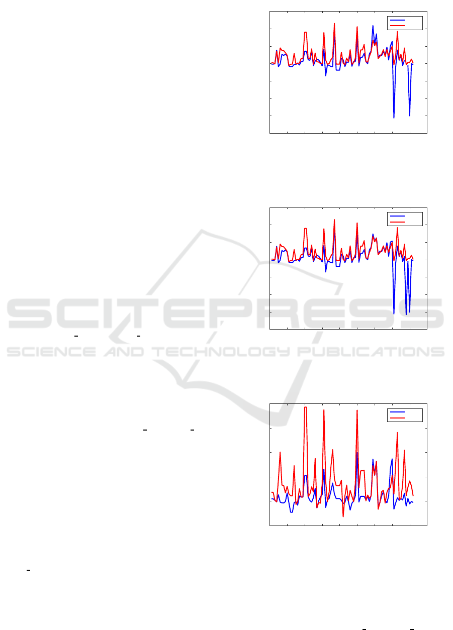
Figure 1 displays the normalized residuals for
examples from the COMPl
e
ib collection, using
MATLAB function
dare
and the standard Newton
solver, with default tolerance and
dare
initialization.
With few exceptions, the Newton solver is either
comparable with
dare
or it improved the normalized
residuals, sometimes by several orders of magnitude.
However, for four examples (HF2D
IS7, HF2D CD5,
HF2D17, and HF2D18, numbered as 59, 61, 69, and
70, respectively, in Fig. 1), clearly worse results have
been obtained. Line search succeeded to get smaller
normalized residuals for these examples, as can be
seen in Fig. 2.
Figure 3 plots the MATLAB-style relative residu-
als for examples from the COMPl
e
ib collection, using
MATLAB function
dare
and Newton solver with line
search, with default tolerance and
dare
initialization.
The Newton solver returned comparable or (much)
smaller residuals except for three examples, namely,
HF2D
IS7, HF2D17, and HF2D18 (numbered as 59,
69, and 70, respectively). For the last two examples,
the standard method gave smaller residuals than the
line search method.
Similarly, Fig. 4 shows the corresponding elapsed
CPU times for the two solvers. For 18 examples, the
0 10 20 30 40 50 60 70 80 90
Example #
10
-35
10
-30
10
-25
10
-20
10
-15
10
-10
10
-5
10
0
Normalized residuals
Normalized residuals for dare and Newton solver
Newton
dare
Figure 1: Normalized residuals for examples from the
COMPl
e
ib collection (taken as discrete-time systems), us-
ing MATLAB function
dare
and standard Newton solver,
with default tolerance and
dare
initialization.
0 10 20 30 40 50 60 70 80 90
Example #
10
-35
10
-30
10
-25
10
-20
10
-15
10
-10
10
-5
10
0
Normalized residuals
Normalized residuals for dare and Newton solver
Newton
dare
Figure 2: Normalized residuals for examples from the
COMPl
e
ib collection, using MATLAB function
dare
and
Newton solver with line search, default tolerance and
dare
initialization.
0 10 20 30 40 50 60 70 80 90
Example #
10
-18
10
-16
10
-14
10
-12
10
-10
10
-8
dare-style residuals
dare-style residuals for dare and Newton solver
Newton
dare
Figure 3: MATLAB-style residuals for examples from the
COMPl
e
ib collection, using MATLAB function
dare
and
Newton solver with line search, default tolerance and
dare
initialization.
computations with standard Newton method ended
before finishing the first iteration, and just six exam-
ples (AGS, PAS, NN11, HF2D
IS7, HF2D CD5, and
ICINCO 2018 - 15th International Conference on Informatics in Control, Automation and Robotics
72
0 10 20 30 40 50 60 70 80 90
Example #
10
-5
10
-4
10
-3
10
-2
10
-1
CPU times (sec)
CPU times for dare and Newton solver
Newton
dare
Figure 4: Elapsed CPU time for examples from the
COMPl
e
ib collection, using MATLAB function
dare
and
standard Newton solver, with default tolerance and
dare
initialization.
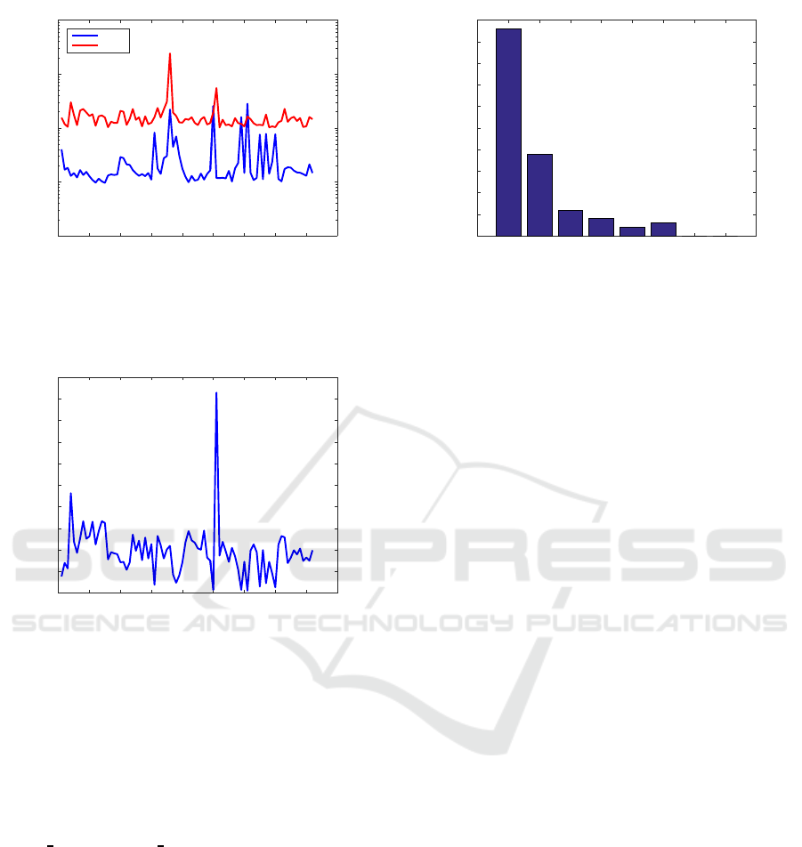
0 10 20 30 40 50 60 70 80 90
Example #
0
5
10
15
20
25
30
35
40
45
50
CPU time ratio
dare CPU time divided by Newton solver CPU time
Figure 5: Ratios of the elapsed CPU time needed by
MATLAB function
dare
and standard Newton solver, with
default tolerance and
dare
initialization, for examples from
the COMPl
e
ib collection.
HF2D17) needed more than one iteration, namely, 8,
11, 11, 50, 50, and 2 iterations, respectively. For the
same examples, the modified Newton method needed
2, 11, 11, 11, 0, and 1 iterations, and it was by
three and two orders of magnitude more accurate for
HF2D
IS7 and HF2D CD5, respectively, and compa-
rable for all other examples. Since very few iterations
are most often needed, the CPU time for the New-
ton solver is a small fraction of that for the MATLAB
solver
dare
. Figure 5 plots the ratios of the elapsed
CPU time needed by MATLAB function
dare
and the
standard Newton solver.
The bar graph from Fig. 6 shows the improvement
obtained using the Newton solver with line search, de-
fault tolerance and
dare
initialization. The height of
the i-th vertical bar indicates the number of examples
for which the improvement was between i−1 and i or-
ders of magnitude, in comparison to
dare
. The num-
ber of examples in the six bins are 48, 19, 7, 2, 5,
1 2 3 4 5 6 7 8
i
0
5
10
15
20
25
30
35
40
45
50
Number of examples
Improvement of dare-style residuals
Figure 6: Bar graph showing the improvement of the
MATLAB-style residuals for examples from the COMPl
e
ib
collection, using Newton solver with line search, default
tolerance and
dare
initialization. The height of the i-th ver-
tical bar indicates the number of examples for which the
improvement was between i-1 and i orders of magnitude.
and 1, corresponding to improvements till one order
of magnitude, between one and two orders of magni-
tude, and so on.
5 CONCLUSIONS
Basic facts and improved procedures and algorithms
for solving discrete-time algebraic Riccati equations
using standard or modified Newton’s method, with
several line search strategies, have been presented.
Numerical results obtained on a comprehensive set
of examples from the COMPl
e
ib collection, taken
as discrete-time systems, have been summarized and
they illustrate the performance and capabilities of this
solver. The possibility to offer, in few iterations, a
reduction by one or more orders of magnitude of the
normalized and MATLAB-style residuals of the solu-
tions computed by MATLAB function
dare
, makes
Newton solver an attractive support tool for solving
DAREs.
ACKNOWLEDGEMENTS
This work was partially supported by the Institu-
tional research programme PN 1819 “Advanced IT re-
sources to support digital transformation processes in
the economy and society — RESINFO-TD” (2018),
project PN 1819-01-01, “New research in complex
systems modelling and optimization with applications
in industry, business and cloud computing”, funded
by the Ministry of Research and Innovation, Roma-
nia.
Numerical Investigation of Newton’s Method for Solving Discrete-time Algebraic Riccati Equations
73

REFERENCES
Abels, J. and Benner, P. (1999a). CAREX—A collection
of benchmark examples for continuous-time algebraic
Riccati equations (Version 2.0). SLICOT Working
Note 1999-14. Available: www.slicot.org.
Abels, J. and Benner, P. (1999b). DAREX—A collection of
benchmark examples for discrete-time algebraic Ric-
cati equations (Version 2.0). SLICOT Working Note
1999-16. Available: www.slicot.org.
Anderson, B. D. O. (1978). Second-order convergent al-
gorithms for the steady-state Riccati equation. Int.
J. Control, 28(2):295–306.
Anderson, B. D. O. and Moore, J. B. (1971). Linear
Optimal Control. Prentice-Hall, Englewood Cliffs,
New Jersey.
Anderson, E., Bai, Z., Bischof, C., Blackford, S., Demmel,
J., Dongarra, J., Du Croz, J., Greenbaum, A., Ham-
marling, S., McKenney, A., and Sorensen, D. (1999).
LAPACK Users’ Guide: Third Edition. Software · En-
vironments · Tools. SIAM, Philadelphia.
Armstrong, E. S. and Rublein, G. T. (1976). A stabiliza-
tion algorithm for linear discrete constant systems.
IEEE Trans. Automat. Contr., AC-21(4):629–631.
Arnold, III, W. F. and Laub, A. J. (1984). Generalized
eigenproblem algorithms and software for algebraic
Riccati equations. Proc. IEEE, 72(12):1746–1754.
Balzer, L. A. (1980). Accelerated convergence of the
matrix sign function method of solving Lyapunov,
Riccati and other matrix equations. Int. J. Control,
32(6):1057–1078.
Benner, P. (1997). Contributions to the Numerical So-
lution of Algebraic Riccati Equations and Related
Eigenvalue Problems. Dissertation, Fakult¨at f¨ur Math-
ematik, Technische Universit¨at Chemnitz–Zwickau,
D–09107 Chemnitz, Germany.
Benner, P. (1998). Accelerating Newton’s method for
discrete-time algebraic Riccati equations. In Beghi,
A., Finesso, L., and Picci, G., editors, Mathemati-
cal Theory of Networks and Systems, Proceedings of
the MTNS-98 Symposium held in Padova, Italy, July,
1998, 569–572. Il Poligrafo, Padova, Italy.
Benner, P. and Byers, R. (1998). An exact line search
method for solving generalized continuous-time alge-
braic Riccati equations. IEEE Trans. Automat. Contr.,
43(1):101–107.
Benner, P., Kressner, D., Sima, V., and Varga, A.
(2010). Die SLICOT-Toolboxen f¨ur Matlab. at—
Automatisierungstechnik, 58(1):15–25.
Benner, P., Mehrmann, V., Sima, V., Van Huffel, S., and
Varga, A. (1999). SLICOT — A subroutine library
in systems and control theory. In Datta, B. N., edi-
tor, Applied and Computational Control, Signals, and
Circuits, vol. 1, ch. 10, 499–539. Birkh¨auser, Boston.
Benner, P. and Sima, V. (2003). Solving algebraic Riccati
equations with SLICOT. In Proceedings of The 11th
Mediterranean Conference on Control and Automa-
tion MED’03, June 18–20 2003, Rhodes, Greece.
Benner, P., Sima, V., and Voigt, M. (2016). Al-
gorithm 961: Fortran 77 subroutines for the so-
lution of skew-Hamiltonian/Hamiltonian eigenprob-
lems. ACM Transactions on Mathematical Software
(TOMS), 42(3):1–26.
Bini, D. A., Iannazzo, B., and Meini, B. (2012). Numeri-
cal Solution of Algebraic Riccati Equations. SIAM,
Philadelphia.
Bunse-Gerstner, A. and Mehrmann, V. (1986). A symplec-
tic QR like algorithm for the solution of the real alge-
braic Riccati equation. IEEE Trans. Automat. Contr.,
AC–31(12):1104–1113.
Byers, R. (1987). Solving the algebraic Riccati equa-
tion with the matrix sign function. Lin. Alg. Appl.,
85(1):267–279.
Chu, E.-W., Fan, H.-Y., and Lin, W.-W. (2005). A structure-
preserving doubling algorithm for continuous-time al-
gebraic Riccati equations. Lin. Alg. Appl., 386:55–80.
Ciubotaru, B. D. and Staroswiecki, M. (2009). Comparative
study of matrix Riccati equation solvers for parametric
faults accommodation. In Proceedings of the 10th Eu-
ropean Control Conference, 23-26 August 2009, Bu-
dapest, Hungary, 1371–1376.
Dongarra, J. J., Du Croz, J., Duff, I. S., and Hammarling, S.
(1990). Algorithm 679: A set of Level 3 Basic Lin-
ear Algebra Subprograms. ACM Trans. Math. Softw.,
16(1):1–17, 18–28.
Gardiner, J. D. and Laub, A. J. (1986). A generalization of
the matrix sign function solution for algebraic Riccati
equations. Int. J. Control, 44:823–832.
Giftthaler, M., Neunert, M., St¨auble, M., and Buchli,
J. (2018). The control toolbox — An open-
source C++ library for robotics, optimal and
model predictive control. [Online]. Available:
https://arxiv.org/abs/1801.04290.
Golub, G. H. and Van Loan, C. F. (1996). Matrix Computa-
tions. The Johns Hopkins University Press, Baltimore,
MA, 3rd edition.
Guo, C. and Laub, A. J. (2000). On a Newton-like method
for solving algebraic Riccati equations. SIAM J. Ma-
trix Anal. Appl., 21(2):694–698.
Guo, C.-H., Iannazzo, B., and Meini, B. (2007). On the
doubling algorithm for a (shifted) nonsymmetric alge-
braic Riccati equation. SIAM J. Matrix Anal. Appl.,
29(4):1083–1100.
Guo, P.-C. (2016). A modified large-scale structure-
preserving doubling algorithm for a large-scale Ric-
cati equation from transport theory. Numerical Algo-
rithms, 71(3):541–552.
Guo, X.-X., Lin, W.-W., and Xu, S.-F. (2006). A structure-
preserving doubling algorithm for nonsymmetric al-
gebraic Riccati equation. Numer. Math., 103(3):393–
412.
Hammarling, S. J. (1982). Newton’s method for solving the
algebraic Riccati equation. NPC Report DIIC 12/82,
National Physics Laboratory, Teddington, Middlesex
TW11 OLW, U.K.
Hewer, G. A. (1971). An iterative technique for the com-
putation of the steady state gains for the discrete op-
timal regulator. IEEE Trans. Automat. Contr., AC–
16(4):382–384.
ICINCO 2018 - 15th International Conference on Informatics in Control, Automation and Robotics
74

J´onsson, G. F. and Vavasis, S. (2004). Solving polynomials
with small leading coefficients. SIAM J. Matrix Anal.
Appl., 26(2):400–414.
Kenney, C., Laub, A. J., and Wette, M. (1989).
A stability-enhancing scaling procedure for Schur-
Riccati solvers. Systems Control Lett., 12:241–250.
Kleinman, D. L. (1968). On an iterative technique for Ric-
cati equation computations. IEEE Trans. Automat.
Contr., AC–13:114–115.
Lancaster, P., Ran, A. C. M., and Rodman, L. (1986). Her-
mitian solutions of the discrete algebraic Riccati equa-
tion. Int. J. Control, 44:777–802.
Lancaster, P., Ran, A. C. M., and Rodman, L. (1987). An
existence and monotonicity theorem for the discrete
algebraic matrix Riccati equation. Lin. and Multil.
Alg., 20:353–361.
Lancaster, P. and Rodman, L. (1980). Existence and unique-
ness theorems for the algebraic Riccati equation. Int.
J. Control, 32:285–309.
Lancaster, P. and Rodman, L. (1995). The Algebraic Riccati
Equation. Oxford University Press, Oxford.
Lanzon, A., Feng, Y., Anderson, B. D. O., and Rotkowitz,
M. (2008). Computing the positive stabilizing solu-
tion to algebraic Riccati equations with an indefinite
quadratic term via a recursive method. IEEE Trans.
Automat. Contr., AC–53(10):2280–2291.
Laub, A. J. (1979). A Schur method for solving algebraic
Riccati equations. IEEE Trans. Automat. Contr., AC–
24(6):913–921.
Leibfritz, F. and Lipinski, W. (2004). COMPl
e
ib 1.0 – User
manual and quick reference. Technical report, Depart-
ment of Mathematics, University of Trier, Trier, Ger-
many.
Mehrmann, V. (1991). The Autonomous Linear Quadratic
Control Problem. Theory and Numerical Solution,
volume 163 of Lect. Notes in Control and Infor-
mation Sciences (M. Thoma and A. Wyner, eds.).
Springer-Verlag, Berlin.
Mehrmann, V. and Tan, E. (1988). Defect correction meth-
ods for the solution of algebraic Riccati equations.
IEEE Trans. Automat. Contr., AC–33(7):695–698.
Pappas, T., Laub, A. J., and Sandell, N. R. (1980). On
the numerical solution of the discrete-time algebraic
Riccati equation. IEEE Trans. Automat. Contr., AC–
25(4):631–641.
Roberts, J. (1980). Linear model reduction and solution of
the algebraic Riccati equation by the use of the sign
function. Int. J. Control, 32:667–687.
Sima, V. (1996). Algorithms for Linear-Quadratic Opti-
mization, volume 200 of Pure and Applied Mathemat-
ics: A Series of Monographs and Textbooks, E. J. Taft
and Z. Nashed (Series editors). Marcel Dekker, Inc.,
New York.
Sima, V. (2013a). Solving discrete-time algebraic Ric-
cati equations using modified Newton’s method. In
6th International Scientific Conference on Physics and
Control, San Luis Potos´ı, Mexico. August 26th-29th,
2013.
Sima, V. (2013b). Solving SLICOT benchmarks for alge-
braic Riccati equations by modified Newton’s method.
In Proceedings of the 17th Joint International Confer-
ence on System Theory, Control and Computing (IC-
STCC 2013), October 11-13, 2013, Sinaia, Romania,
491–496. IEEE.
Sima, V. (2014). Efficient computations for solving alge-
braic Riccati equations by Newton’s method. In Mat-
covschi, M. H., Ferariu, L., and Leon, F., editors, Pro-
ceedings of the 2014 18th Joint International Confer-
ence on System Theory, Control and Computing (IC-
STCC 2014), October 17-19, 2014, Sinaia, Romania,
609–614. IEEE.
Sima, V. (2015). Computational experience with a modified
Newton solver for continuous-time algebraic Riccati
equations. In Ferrier, J.-L., Gusikhin, O., Madani, K.,
and Sasiadek, J., editors, Informatics in Control Au-
tomation and Robotics, volume 325 of Lecture Notes
in Electrical Engineering, ch. 3, 55–71. Springer In-
ternational Publishing.
Sima, V. and Benner, P. (2006). A SLICOT imple-
mentation of a modified Newton’s method for alge-
braic Riccati equations. In Proceedings of the 14th
Mediterranean Conference on Control and Automa-
tion MED’06, June 28-30 2006, Ancona, Italy. Omni-
press.
Sima, V. and Benner, P. (2008). Experimental evaluation of
new SLICOT solvers for linear matrix equations based
on the matrix sign function. In Proceedings of 2008
IEEE Multi-conference on Systems and Control. 9th
IEEE International Symposium on Computer-Aided
Control Systems Design (CACSD), San Antonio, TX,
U.S.A., September 3–5, 2008, 601–606. Omnipress.
Sima, V. and Benner, P. (2014). Numerical investigation
of Newton’s method for solving continuous-time al-
gebraic Riccati equations. In Ferrier, J.-L., Gusikhin,
O., Madani, K., and Sasiadek, J., editors, Proceedings
of the 11th International Conference on Informatics in
Control, Automation and Robotics (ICINCO-2014), 1-
3 September, 2014, Vienna, Austria, vol. 1, 404–409.
SciTePress.
Sima, V. and Benner, P. (2015). Solving SLICOT bench-
marks for continuous-time algebraic Riccati equa-
tions by Hamiltonian solvers. In Proceedings of the
2015 19th International Conference on System The-
ory, Control and Computing (ICSTCC 2015), October
14-16, 2015, Cheile Gradistei - Fundata Resort, Ro-
mania, 1–6. IEEE.
Van Dooren, P. (1981). A generalized eigenvalue approach
for solving Riccati equations. SIAM J. Sci. Stat. Com-
put., 2(2):121–135.
Van Huffel, S., Sima, V., Varga, A., Hammarling, S., and
Delebecque, F. (2004). High-performance numeri-
cal software for control. IEEE Control Syst. Mag.,
24(1):60–76.
Numerical Investigation of Newton’s Method for Solving Discrete-time Algebraic Riccati Equations
75
