Forecasting the Class of Daily Clearness Index for PV Applications

Giuseppe Nunnari

Dipartimento di Ingegneria Elettrica, Elettronica e Informatica, Universit

a degli Studi di Catania,

Viale A. Doria, 6, 95125 Catania, Italy

Keywords:

Clearness Index, Hidden Markov Models, Neural Network Models, Naive-Bayes Models, Surrogate Models,

Persistent Model.

Abstract:

This paper deals with the problem of forecasting the class of the daily clearness index which can be relevant

for PV applications. A large number of solar stations, publicly available, was processed by using ﬁve different

approaches, namely, the feed-forward neural networks, the Hidden Markov models, the Naive-Bayes models,

the Surrogate models and the Persistent models. Experimental results show that one-day ahead forecasting of

the class of daily clearness can be reliable performed in a 2-class framework and with less accuracy in a 3-class

framework. Furthermore, for this purpose, the HMM approach is recommended among the considered ones.

The global performance of the class prediction models, evaluated by calculating the average confusion rate

(CR), showed that using HMM models provide C R ≤ 0.3 for 2-class clustering classes, while, for the 3-class

framework it rises to 0.35.

1 INTRODUCTION

Solar energy is a source of clean energy of ever in-

creasing interest, with the feature of being ﬂoating

at all-time scales. As the weight of the photovoltaic

plants (PV) becomes more consistent over the whole

electricity production grid, it is obvious that the prob-

lem of energy ﬂuctuations becomes increasingly im-

portant for the purposes of the grid stability. The in-

termittent and stochastic character of solar radiation

has been studied for instance by (Notton and Voyant,

2018). A recent review paper who tries to identify-

ing methods that may be used to forecast PV power

ﬂuctuations is given by (Barbieri et al., 2017). One of

the approaches to reduce the impact of ﬂuctuations

is prediction. Indeed, this allows managers to bal-

ance the production of electrical energy by using con-

ventional sources (Antonanzas et al., 2016). A huge

literature referring with the problem of solar radia-

tion forecast, demonstrates that statistical approaches,

mainly of autoregressive kinds, are able to predict so-

lar energy at very-short term only, as clearly stated in

(Voyant et al., 2017). Indeed, in the very short time

domain, referred to as Now-casting (0 -3 h), the fore-

cast is usually based on extrapolations of real-time

measurements, while for Short-Term Forecasting (3

- 6 h), real-time measurements or satellite data are

coupled with Numerical Weather Prediction (NWP)

models.

A huge plethora of approaches for short-term predic-

tion of solar radiation time series have been proposed

which include, Artiﬁcial Neural Networks (ANN)

(Raza et al., 2018), Adaptive Neuro-Fuzzy Infer-

ence Systems (ANFIS) (Piri and Kisi, 2015), Par-

ticle Swarm Optimization and Evolutionary algo-

rithms (Nian et al., 2013), Generalized Autoregres-

sive with Conditional Heteroskedasticity (ARMA-

GARCH) models (Sun et al., 2015), Bayesian sta-

tistical models (Lauret et al., 2013), Fuzzy coupled

with Genetic Algorithms models (Kisi, 2014), just to

mention a few. Furthermore, statistical approaches

based on decomposition of the original time series

have been studied in (Prema and Rao, 2015). How-

ever, regardless of the considered approach, statistical

(autoregressive) models, since are based on the natu-

ral autocorrelation of measures performed at a point,

cannot reliably forecast the exact value of solar ra-

diation at daily scale, i.e. 1-day ahead. To partially

overcome this shortcoming, we propose in this paper

to modify the target of forecasting from true to class

values. In other words, we propose to associating to

the original solar radiation time series, a time series of

classes c(t), i.e. a sequence of integer values, which

will become the forecasting target. It is trivial to un-

derstand that this kind of forecasting problem is as

much hard as large is the number of classes associ-

172

Nunnari, G.

Forecasting the Class of Daily Clearness Index for PV Applications.

DOI: 10.5220/0006860801720179

In Proceedings of the 15th International Conference on Informatics in Control, Automation and Robotics (ICINCO 2018) - Volume 1, pages 172-179

ISBN: 978-989-758-321-6

ated to the original time series. For this reason, in this

paper we will consider clustering into 2 or 3 classes.

Furthermore, in order to avoid dealing directly with

the amount of solar radiation, we consider the clear-

ness index, a dimensionless measure of the solar radi-

ation at ground level, deﬁned as (1).

clr

(1)

In expression (1), I

is the solar radiation irradiance

measured at ground level and I

clr

is the modeled clear

sky irradiance. Computing the clearness index, we ﬁl-

ter the deterministic ﬂuctuation of solar radiation due

to the natural Earth’s rotation and spinning, thus leav-

ing the random component generated by weather con-

ditions and in particular by the clouds cover. Among

several clear sky models proposed in literature to

compute the I

clr

term, we have considered the Ine-

ichen and Perez model for global horizontal irradi-

ance, as presented in (Ineichen and Perez, 2002) and

(Perez, 2002). The Matlab code that implement this

model was belongs to the SNL PVLib Toolbox, is-

sued by the Sandia National Labs PV Modeling Col-

laborative (PVMC) platform. This paper is organized

as follows. In section 2 we will report some results

concerning the analysis of daily k

time series with the

aim of showing that they represent a hard task for au-

toregressive models, since they are based on the nat-

ural autocorrelation. In section 3 we will give a brief

description of the machine learning approaches con-

sidered to perform forecasting. Section 4 is devoted

to describe numerical results and, ﬁnally, in section 5

we draw some conclusions.

2 ANALYSIS OF DAILY

CLEARNESS TIME SERIES

In order to objectively characterize the behavior of

daily k

time series, several analyzes were carried out

on a representative set of solar radiation recording sta-

tions.

2.1 Data and Sites

To make reproducible the results described in this pa-

per, public available data was considered. Indeed,

the data set consists of hourly average time series

recorded at hundreds stations stored in the National

Solar Radiation Database managed by the NREL (Na-

tional Renewable Energy Laboratory). Data of this

database was recorded from 1991 to 2005. It is rather

difﬁcult to give a precise idea of the variability of this

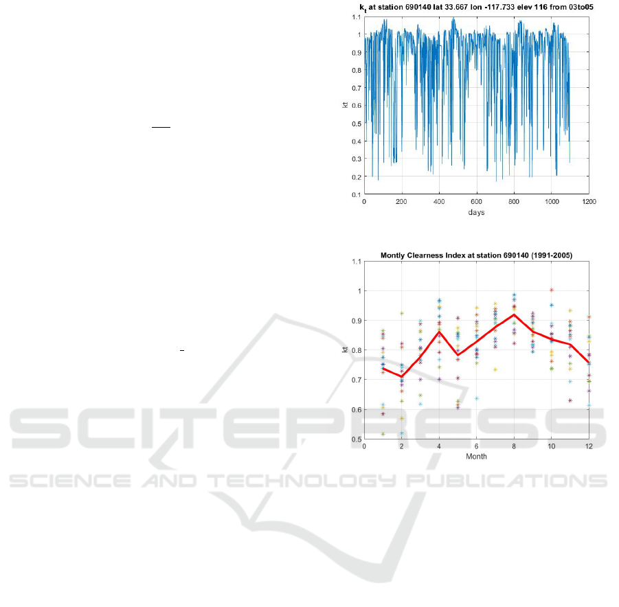
Figure 1: k

daily values computed at the station ID690140.

Figure 2: Fluctuations of the monthly k

index the station

ID690140 during 1991 to 2015.

type of time series as it depends very much on the ge-

ographical location, and particularly on the latitude.

However, just to familiarize, we report in Figure 1

daily values of k

measured at the station ID690140

from 2003 to 2005. It can be seen that there is a

high variability of this index at daily time scale, with

the feature that during summer months the range of

variability is lower with respect to the others months.

However, large k

ﬂuctuations occurs from month to

month and for each month, as shown in Figure 2.

The dots represent the monthly k

values, averaged

for each month of the year from 1991 to 2005, while

the thick red curve is obtained averaging over each

month.

2.2 Slope of the k

Power Density

Spectrum

The absolute value of the slope of the power den-

sity spectrum, here indicated as β, is often considered

to characterize the long-term memory of a process.

For instance, a slope equal to zero indicates a white

Forecasting the Class of Daily Clearness Index for PV Applications

173

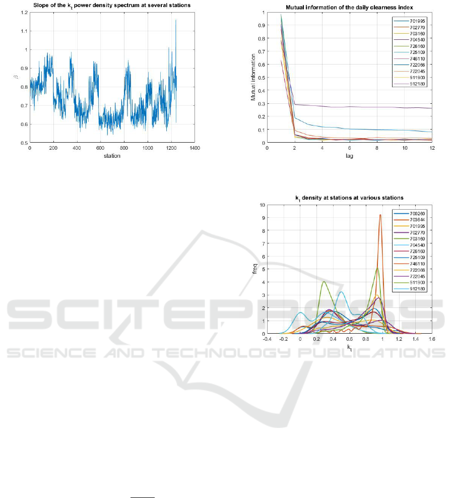
Figure 3: Slope of k

daily values power density spectrum

computed for several hundreds stations of the dataset.

noise, i.e. a completely uncorrelated time series, due

to the fact that its energy is equally distributed for all

frequencies and thus the power spectrum is ﬂat. In-

stead, a random walk, i.e. a time series in which the

differences between consecutive samples is a white

noise, has β = 2. A slope ranging between β = 0.5

to β = 1.5 is a signature of the so-called 1/ f noise.

Long-memory processes have been observed in sev-

eral ﬁelds such as physics, biology, astrophysics, geo-

physics, and sociology, just to mention a few.

We have computed the slope of daily k

density spec-

trum for several hundred of stations, as shown in Fig-

ure 3. As it is possible to see, β ranges in [0.5,1.2],

with an average value of about 0.63, thus meaning that

daily k

time series can be classiﬁed as 1/ f noises.

2.3 Mutual information

Since, dealing with the traditional autocorrelation

function one of the shortcomings is that it is a linear

measure, in this paper, in order to capture the nonlin-

ear correlation of daily k

time series, we have com-

puted the so called mutual information I, deﬁned as

(2).

I = −

∑

i, j

i j

(k)ln

i j

(k)

(2)

In this expression, for some partition of the time se-

ries range, p

is the probability to ﬁnd a time series

values in the i

interval and p

i j

is the joint probabil-

ity that an observation falls in the i

interval and the

observation time k later falls into the j

interval.

The Mutual information computed for a selected

number of stations in a wide range of latitudes is

shown in Figure (4). It is possible to see, regard-

less the particular station, that it decays from 1 to

0.1 in approximately one lag, thus meaning that it is

Figure 4: Mutual information of k

daily values computed

for selected station operating in a wide range of latitudes.

Figure 5: k

densities at 12 station with different latitude in

the range lat ∈ [13.5670,70.2170]. The station in the top of

the legend has lat = 70.2170, while the one at the bottom

has latitude lat = 13.5670. The others station differs each

other about 5 degrees in terms of latitude.

rather difﬁcult to reliably forecast the k

index, one-

day ahead, by using Auto-regression models only.

2.4 k

Probability Distribution Densities

Functions

The probability distribution densities function (pdf)

of daily k

is strictly depending on the geographical

coordinates of the measuring station and in particular

on the latitude, as shown in Figure 5. Roughly speak-

ing, it is possible to say that solar stations located at

high latitudes exhibit pdf density functions with peaks

at low k

value. Furthermore, stations with latitude in

a narrow interval, exhibits densities with peaks in a

narrow k

interval, as shown in Figure 6.

ICINCO 2018 - 15th International Conference on Informatics in Control, Automation and Robotics

174

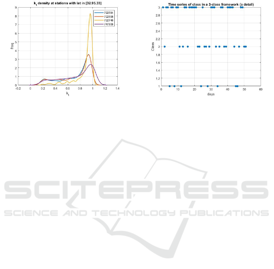
Figure 6: k

densities at four station with latitude in a narrow

range ∈ [32.95,33].

3 FORECASTING THE CLASS OF

DAILY CLEARNESS

Predicting the class of k

does require the replacement

of the original time series with an integer time se-

ries c(t), referred to as a time series of classes. Of

course, the prediction problem is as difﬁcult as larger

the number of considered classes.

3.1 Associating a Time Series of Classes

to Daily Clearness

Among several criteria available to associate a time

series of classes to daily k

, we have considered in this

paper a simple threshold based approach. In more de-

tail we set a threshold equal to 0.70 for clustering into

two classes and the thresholds [0.6,0.8] when we in-

tend to cluster into three classes. These values were

experimental computed in order to roughly balance

the number of elements in each class. Probably, this

criterion is too simplistic for solar stations operating

in a wide range of latitudes. However, since this is a

preliminary study of and we aim to have a rough idea

of predictability of the k

class, we believe that this

choice is acceptable. Clustering into two and three

classes k

time series, will be referred in the paper as

2-class and 3-class framework, respectively. An ex-

ample of time series of the class in a 3-class frame-

work is shown in Figure 7.

3.2 Machine Learning Approaches

We have considered three popular machine learn-

ing approaches, namely the Hidden Markov Model

(HMM), the Non-linear Autoregressive (NAR) model

and the Naive Bayesian model (NBM) in order to

Figure 7: Time series of classes associated to k

daily time

series, recorded at the station 690140 (a detail).

solve the stated forecasting problem. Furthermore,

we have inter-compared the performances with two

different kinds of low reference models, namely the

persistent and the surrogate model. These models are

shortly described in the following sections.

3.3 Predicting the Class by using HMM

Models

A HMM (Rabiner, 1989) is a modeling approach in

which we observe a sequence of emissions, but we

do not know the sequence of states the model went

through to generate the emissions. Thus, in general

a HMM model is characterized by two matrices, re-

ferred to as the transition and the emission matrices,

respectively. In our schematization, we consider the

true time-series of classes c(t) associated to k

, as the

sequence of states and the sequence of classes ob-

served for tomorrow, i.e. c(t + 1), as the sequence

of emissions. Based on these assumptions, we train

a HMM model to forecast ˆc(t + 1). To transform

the transition and emission matrices, computed dur-

ing the training process, into the sequence of classes

ˆc(t + 1), we have considered the Viterbi algorithm

(Viterbi, 1967).

3.4 Predicting the Class by using NAR

Models

The NAR-based model consists of two main steps.

1. In the ﬁrst step, one-day ahead k

predictions are

performed by using a non-linear regression model

of the form (3).

(t + 1) = f (k

(t), k

(t − 1),..., k

(t − (d − 1))

(3)

Forecasting the Class of Daily Clearness Index for PV Applications

175

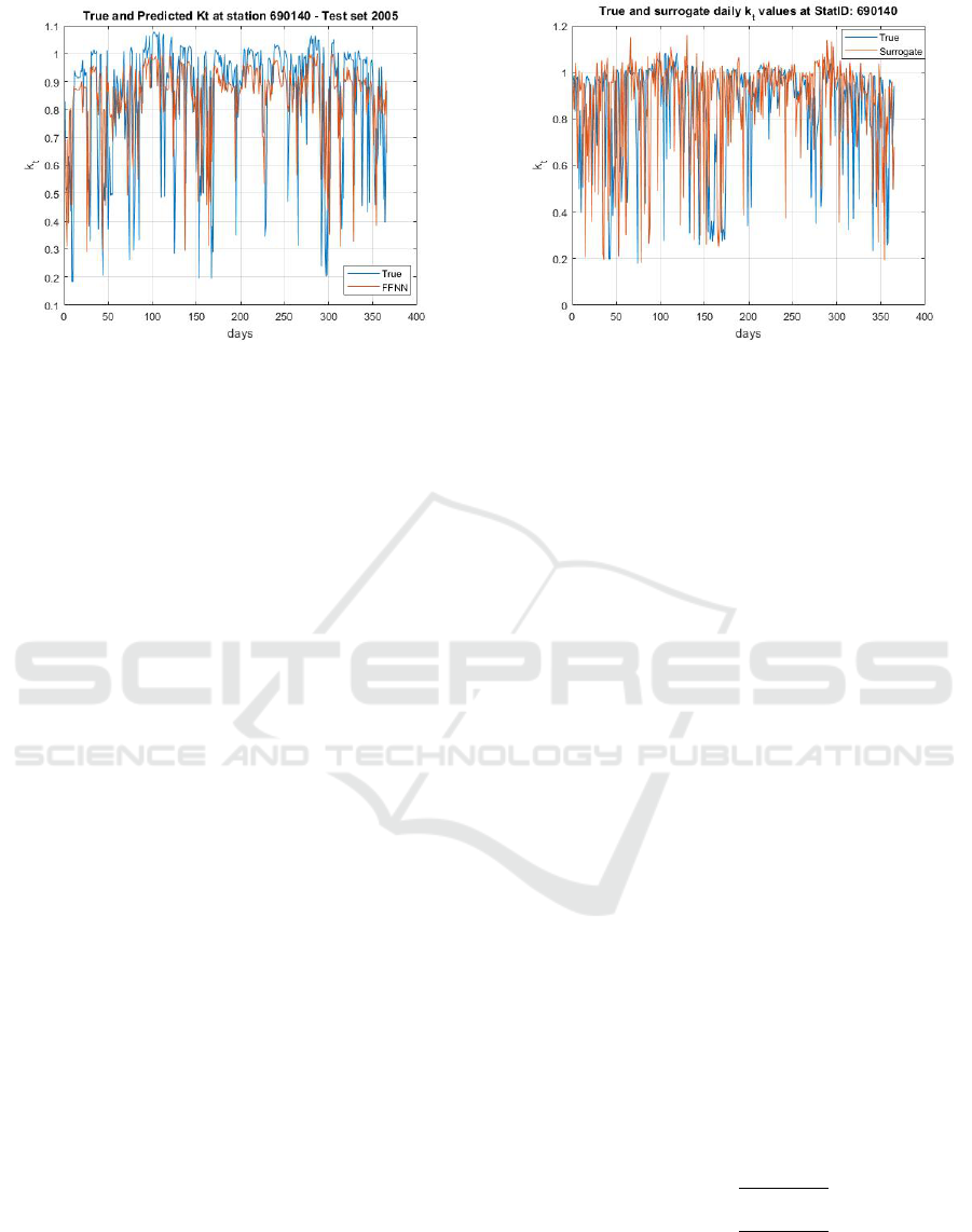
Figure 8: True-Predicted k

at the station 690140.

2. In the second step, the predicted class ˆc(t + 1) is

obtained by associating a class to the predicted

(t + 1), as described in section 3.1.

In this paper, step 1 was performed by training a feed-

forward neural network (FFNN), to approximate the

unknown non linear function f . The number of delays

d in expression (3) was set to 2, due to the scarce auto-

correlation of the daily k

clearness index, as pointed

out in section 2.3. The FFNN was trained by using k

values, recorded during 2003-2014, while the test was

performed considering the year 2005. As an example,

the true and predicted values at the station ID690140

are shown in Figure 8. For all trials the number of

neurons of the FFNN in a unique hidden layer was set

to 20.

3.5 Predicting the Class by using Naive

Bayes Classiﬁer

Naive Bayes classiﬁers are probabilistic classiﬁers

based on the Bayes theorem, with a strong (naive)

independence assumption between the features. In

more detail, indicating as f (x) a classiﬁer that maps

the input features x ∈ X to the output class label

y ∈ {1,...,n

}, a Naive Bayes classiﬁer is character-

ized by expression (4).

f (x) = ˆy(x) = argmax

p(y|x) (4)

where p(y|x) is the class posterior probability density

which is computed by applying the Bayes rule.

3.6 Predicting the Class by using Low

Level Reference Models

In this paper, we consider two low reference models

to predict the class of k

, namely the persistent model

and the surrogate models.

Figure 9: True and surrogate daily k

values at the station

690140.

3.6.1 The Persistent Model

The persistent model forecasts the class by using the

equation ˆc(t + 1) = c(t).

3.6.2 The Surrogate Model

With the term surrogate model we refer one which

generates

(t) by using a kernel function trough the

following steps:

• let p

the probability density function (pdf) of k

computed by using a kernel function;

• generate a time series

(t) of random number

having p

as pdf, which will be considered as

forecast;

• associate a time series of class to

(t).

In this paper, in order to generate more realistic sur-

rogate time series, instead of using a unique p

pdf

function, we have identiﬁed, for each individual sta-

tion, 12 different functions, one for each month of the

year. An example of true and surrogate k

time series

is shown in Figure 9.

3.7 Performance Indices

In order to objectively asses to what extent a predicted

time series of classes is close to the true one, we have

considered the T PR (True Predicted Rate) and the

T NR (True Negative Rate), deﬁned as follows:

T PR(i) =

T P(i)

T P(i)+FN(i)

(5)

T NR(i) =

T N(i)

T N(i)+FP(i)

(6)

where T P(i) and FN(i) is the number of true posi-

tive and false positive patterns, respectively, attributed

by the model to the class C

and i is the class in-

dex. The sum P(i) = T P(i) + FN(i) is, of course,

ICINCO 2018 - 15th International Conference on Informatics in Control, Automation and Robotics

176

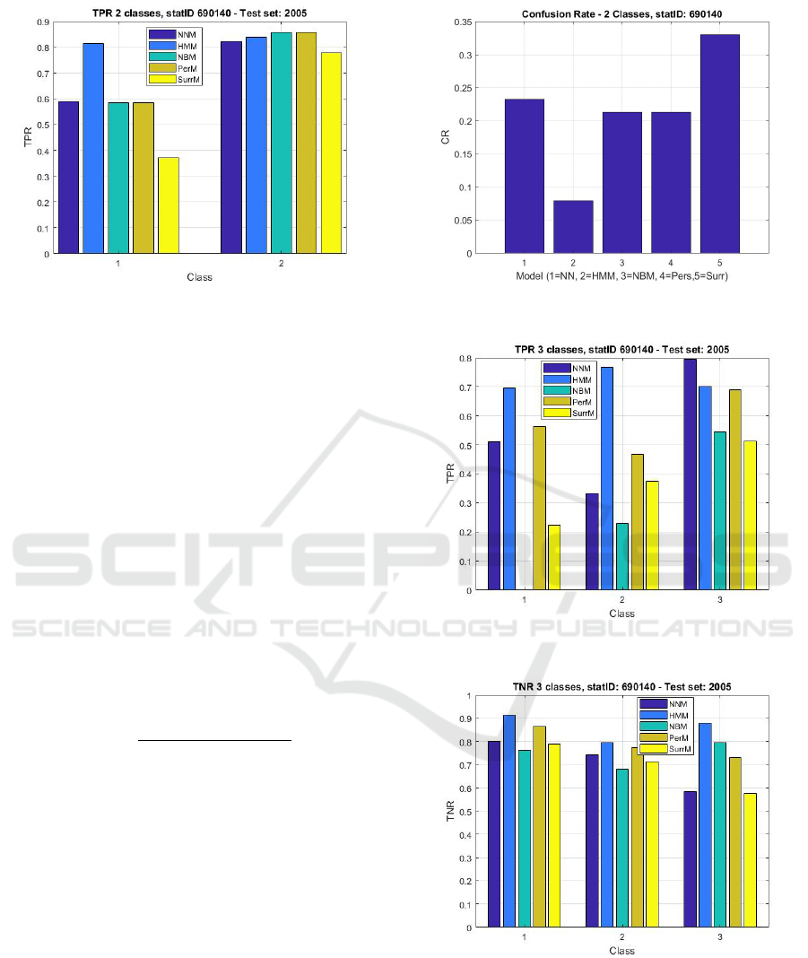
Figure 10: TPR for the 2-class framework at the station

ID690140.

the total number of patterns attributed by the model

to the class C

. Similarly, T N(i) is the number of pat-

terns which are correctly identiﬁed as not belonging

to the class C

and FP(i) is the number of false posi-

tives attributed by the model to the class C

. The sum

N(i) = T N(i) + FP(i) is the total number of patterns

recognized by the model as not belonging to the class

. Clearly, a good predictor would be characterized

by values of TPR and TNR both close to 1. Further-

more, it is to bearing in mind that for a 2-class frame-

work equations (7) hold.

T NR(1) = T PR(2) (7)

T NR(2) = T PR(1) (8)

As a global index, to measure the classiﬁer perfor-

mances, we have computed the so-called confusion

rate index CR, deﬁned as (9):

CR =

FP + FN

T P + T N + FP + FN

(9)

Of course CR ∈ [0,1] and lower values of c

are best.

4 NUMERICAL RESULTS

Results described in this section was obtained by us-

ing, for each station, time series, recorded from 2003

to 2005. Two years of data (2003 and 2004) was con-

sidered to identify the models, while the remaining for

the test. As an example, referring to a 2-class frame-

work, the performances of the ﬁve inter-compared

models, in terms of TPR and CR, are shown in Figure

10 and 11, respectively. As it is possible to see, the

HMM model outperform the others, since exhibits a

TPR better than 0.8 for both the classes and a confu-

sion rate better than 0.1. Similarly, clustering into

three classes, the performances of the inter-compared

Figure 11: CR for the 2-class framework at the station

ID690140.

Figure 12: TPR in a 3-class clustering at the station

ID690140.

Figure 13: TNR in a 3-class clustering at the station

ID690140.

approaches are shown in Figure 12,13 and 14 respec-

tively. As it is possible to see, even if the HMM

approach is not the best in terms of TPR for all the

classes, since for instance for the class C

the NNM

model outperform the others (Figure 12), it is the one

Forecasting the Class of Daily Clearness Index for PV Applications

177

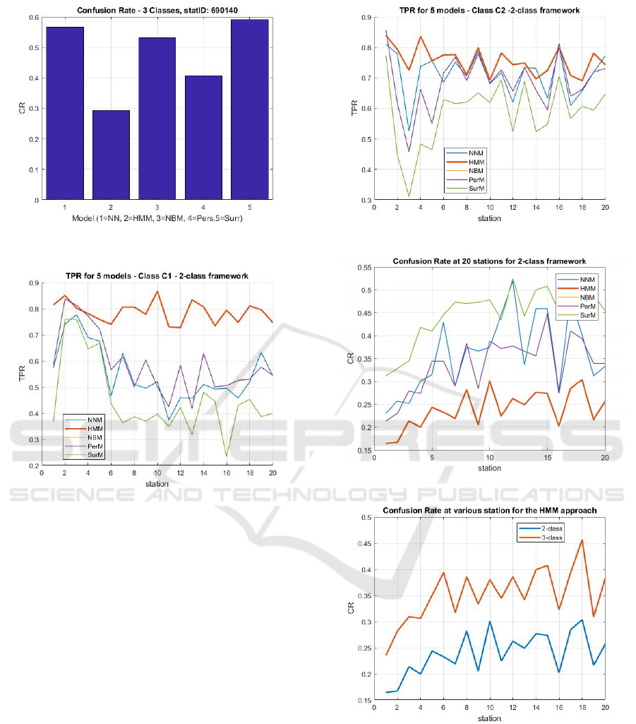
Figure 14: CR in a 3-class framework, at the station

ID690140.

Figure 15: TPR at 20 stations, for the class C1.

which exhibits the lowest CR, that, for this station, is

lower than 0.3 (see Figure 14).

As we are aware that results obtained for an indi-

vidual station do not allow to draw general conclu-

sions, we have repeated the calculations for several

stations of the NOAA database. In Figure 15, 16

and 17, we report the results, in terms of TPR and

CR, for 20 stations selected in a wide range of lati-

tudes, for a 2-class framework. To simplify the Fig-

ures, the selected stations are indicated by integers

from 1 to 20. As it is possible to see, the HMM

model exhibits, with rare exceptions, the best TPR,

as shown in Figure 15 and 16 for the classes C

and C

, respectively. Furthermore, the HMM ap-

proach exhibits the lowest CR (see Figure 17). In

more detail, for the 2-class framework, we have com-

puted, averaging among the 20 stations, that the mean

confusion rates are: 0.3607,0.2385,0.3350,0.3350,

and 0.44567 for the NNM, HMM, NBM, PerM and

SurM models, respectively. Thus, the HMM is the

best, among the ﬁve inter-compared models, in terms

of CR, while the SurM is the worst. As obvious,

Figure 16: TPR at 20 stations, for the class C2.

Figure 17: CR at 20 stations, for the 2-class framework.

Figure 18: CR comparison, for the 2-class and 3-class

frameworks, at 20 stations.

the CR increases when we try to forecast in a 3-

class framework, as shown in Figure 18. For the

3-class framework, we have computed, averaging

among the 20 stations, the following confusion rates:

0.5116,0.3515, 0.4820,0.4613, 0.5708, for the NNM,

HMM, NBM,PersM and SurrM, respectively. Thus,

it is conﬁrmed that also in this case the HMM model

ICINCO 2018 - 15th International Conference on Informatics in Control, Automation and Robotics

178

outperforms the others. However, as expected, the

mean confusion rate rises to 0.3515, while, as de-

scribed above, for the 2-class framework it is 0.2385.

5 CONCLUSIONS

This work was motivated by the awareness that one-

day ahead forecasting of k

time series cannot be re-

liably performed by using autoregressive models, due

to the lack of autocorrelation at daily scale, as pointed

out in section 2. To overcome this drawback, we tried

to perform 1-step ahead forecasting of the k

class.

To this purpose, we have implemented ﬁve different

forecasting models. One of them is still a nonlinear

autoregressive model (NNM), while two are proba-

bilistic (the HMM and the NMB). Finally, the two re-

maining are the well-known persistent model (PersM)

and the surrogate model (SurM), based on the genera-

tion of random sequences with predeﬁned probability

density functions. Results, obtained processing time

series of a signiﬁcant number of recording stations,

point out that forecasting 1-step ahead the class of

daily k

in a 2-class framework can be done with rel-

ative high accuracy. In other terms, we can forecast if

the daily k

for tomorrow, will be lower or higher than

the threshold value, that in this paper was assumed to

be equal to 0.70, for all the stations. For this purpose,

based on our experience, we recommend the HMM

approach which gives CR ≤ 0.3, for all the stations,

with an average value of about 0.25. Forecasting in

a 3-class framework is still possible but with lower

accuracy, since the CR is, on average, of about 0.35.

However, we believe that improvements are possible

by incorporating into the models some peculiar fea-

tures of the individual stations (e.g. the latitude), an

aspect that in this work has not been taken into ac-

count. Indeed, as we have seen in section 2.4, k

prob-

ability density functions are strictly related to latitude

and therefore a classiﬁcation with ﬁxed thresholds, as

done in this work, can not guarantee the best results.

Work is in progress to this end.

REFERENCES

Antonanzas, J., Osorio, N., Escobar, R., Urraca, R., de Pi-

son, F. M., and Antonanzas-Torres, F. (2016). Re-

view of photovoltaic power forecasting. Solar Energy,

136:78 – 111.

Barbieri, F., Rajakaruna, S., and Ghosh, A. (2017). Very

short-term photovoltaic power forecasting with cloud

modeling: A review. Renewable and Sustainable En-

ergy Reviews, 75:242 – 263.

Ineichen, P. and Perez, R. (2002). A new airmass inde-

pendent formulation for the linke turbidity coefﬁcient.

Physica A, 73:151–157.

Kisi, O. (2014). Modeling solar radiation of mediterranean

region in turkey by using fuzzy genetic approach. En-

ergy Conversion and Management, 64:429–436.

Lauret, P., Boland, J., and Ridley, B. (2013). Bayesian sta-

tistical analysis applied to solar radiation modelling.

Renewable Energy, 49:124–127.

Nian, Z., Behera, P., and Williams, C. (2013). Solar ra-

diation prediction based on particle swarm optimiza-

tion and evolutionary algorithm using recurrent neu-

ral networks. IEEE International Systems Conference

(SysCon) 2013.

Notton, G. and Voyant, C. (2018). Chapter 3 - forecasting

of intermittent solar energy resource. In Yahyaoui, I.,

editor, Advances in Renewable Energies and Power

Technologies, pages 77 – 114. Elsevier.

Perez, R. (2002). A new operational model for satellite-

derived irradiances: Description and validation. Solar

Energy, 73:307–317.

Piri, J. and Kisi, O. (2015). Modelling solar radiation

reached to the earth using anﬁs, nn-arx, and empirical

models (case studies: Zahedan and bojnurd stations).

Journal of Atmospheric and Solar-Terrestrial Physics,

123:39–47.

Prema, V. and Rao, K. U. (2015). Development of statistical

time series models for solar power prediction. Renew-

able Energy, 83:100–109.

Rabiner, L. R. (1989). A tutorial on hidden markov models

and selected applications in speech recognition. Math-

ematics of Control, Signals, and Systems, 77:257–286.

Raza, M. Q., Mithulananthan, N., and Summerﬁeld, A.

(2018). Solar output power forecast using an ensemble

framework with neural predictors and bayesian adap-

tive combination. Solar Energy, 166:226 – 241.

Sun, H., Yan, D., Zhao, N., and Zhou, J. (2015). Empirical

investigation on modeling solar radiation series with

armagarch models. Energy Conversion and Manage-

ment, 92:385–395.

Viterbi, A. J. (1967). Error bounds for convolutional codes

and an asymptotically optimum decoding algorithm.

IEEE Transactions on Information Theory, 13:260–

269.

Voyant, C., Notton, G., Kalogirou, S., Nivet, M., Paoli, C.,

Motte, F., and Fouilloy, A. (2017). Machine learning

methods for solar radiation forecasting - a review. Re-

newable Energy, 105:569–582.

Forecasting the Class of Daily Clearness Index for PV Applications

179