Water Asset Management Strategy based on Predictive Rainfall/Runoff

Model to Optimize the Evacuation of Water to the Sea

Baya Hadid and Eric Duviella

Institut Mines Telecom Lille Douai, Univ. Lille, France

Keywords:

Modelling, Water Management, Rainfall/Runoff Model, Optimization, Large Scale Systems, Water System.

Abstract:

Hydrographical networks are large scale systems that are used to answer to the Human uses. They are impacted

by extreme events that should be bigger due to climate change. By focusing on extreme rainy events, the

amount of water in excess has to be dispatched on all the network to avoid ﬂood, and then rejected to the sea

heeding the tides. Pumps can also be used to reject the water to the sea but they lead to big operating cost. To

deal with this challenging issue, the modelling tools and the water asset management strategies that have been

recently proposed are adapted and improved in this paper. They consist in an integrated model, a ﬂow-based

network and a quadratic optimization based on constrains. The efﬁciency of this water management strategy

requires an accurate predictive rainfall/runoff model. It is highlighted by considering a realistic case study that

is also used to describe all the methodology step.

1 INTRODUCTION

Transport via inland waterways beneﬁts of econo-

mic and environmental advantages (Kara et al., 2015;

Mihic et al., 1993; Mallidis et al., 2012; Brand

et al., 2012). However, the inland waterways will

be strongly impacted by climate hazards (Koetse and

Rietveld, 2009; EnviCom, 2008; IWAC, 2009). It is

conﬁrmed by the studies in (Arkell and Darch, 2006),

(Wang et al., 2007) and (Jonkeren et al., 2007) that fo-

cus on inland waterways in UK, in China and on the

Rhine respectively. The frequency and intensity of

future ﬂood events are expected higher (Bates et al.,

2008; Bo

e et al., 2009; Ducharne et al., 2010). To

deal with the management of inland waterways in a

climate change context, a multi-scale management ar-

chitecture has been proposed in (Duviella et al., 2013)

and developed in (Nouasse et al., 2016b), allowing the

use of modelling approaches and management stra-

tegies for water level control (Segovia et al., 2017;

Horv

ath et al., 2014b; Horv

ath et al., 2015a; Horv

ath

et al., 2015b; Rajaoarisoa et al., 2014), and water vo-

lume allocation (Nouasse et al., 2015; Nouasse et al.,

2016a). However, it has been shown that even if it

is possible to control the hydraulic structures with ef-

ﬁciency by considering a deterministic problem, un-

controlled intakes and withdrawals have a strong in-

ﬂuence on this optimization. It is particularly the case

for rainy events that have big inﬂuence on inland wa-

terways. Moreover, inland waterways with outlet to

the sea have not been considered. This implies a new

challenging issue that requires to take into account the

effect of the tide and the electrical cost of the pumps

during the design of the water management strategies.

The management strategy that consists in an opti-

mal adaptive allocation planning of water resource is

adapted and improved in this paper by dealing with

inland waterways with outlet to the sea. The inﬂu-

ence of the tide has taken into account. A criterion

to minimize is deﬁned based on the conﬁguration of

the inland waterways, the priorities on water inta-

kes and withdrawals, the management objectives, the

tide and the predicted volumes that come from rainy

events. The requirement of an accurate prediction of

the amount of water volumes that comes from rain is

highlighted by considering a realistic case study.

The modelling tools and the optimal allocation

planning approach are described in the ﬁrst section.

In the second section, a state of the art of existing pre-

dictive rainfall/runoff models is presented. Then, a

case study allows illustrating all the step to implement

the designed tools and strategy is proposed in the third

section. This case study is used to highlight the im-

portance of the rainfall/runoff models during the opti-

mization of the water resource planning.

Hadid, B. and Duviella, E.

Water Asset Management Strategy based on Predictive Rainfall/Runoff Model to Optimize the Evacuation of Water to the Sea.

DOI: 10.5220/0006866500760085

In Proceedings of the 15th International Conference on Informatics in Control, Automation and Robotics (ICINCO 2018) - Volume 1, pages 76-85

ISBN: 978-989-758-321-6

2 WATER ASSET MANAGEMENT

STRATEGY

2.1 Integrated Model

An integrated model that is linked with a ﬂow-based

network has been proposed in (Nouasse et al., 2016b)

to deal with inland navigation networks. It aims at

modelling the dynamics of each Navigation Reach

(NR), i.e. a part of the canal located between two

locks, as a tank with a sample time of several hours. It

allows taking into account all the inputs and outputs,

controlled or not, of each NR. For inland waterways

with links to the sea, it is necessary to deﬁne a new

element representing the output of the integrated mo-

del. The model consists in considering a ﬁnite number

η of interconnected NR that are linked following the

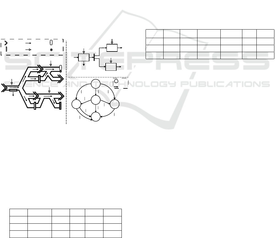
conﬁguration of the network (see Figure 1.a). Each

NR is numbered and denoted NR

, with i ∈ 1 to η.

(a)

Lock

i-2

i-1

i+1

i+2

(b)

i-2

i-1

i+1

i+2

s,c

e,c

g,u

i-2

s,c

i-2

e,c

i-2

g,u

i-1

s,c

i-1

e,c

i-1

g,u

i+1

s,c

i+1

e,c

i+1

g,u

i+2

s,c

i+2

o,c

i+2

g,u

i-2

s,p

i-2

e,p

i-1

s,p

i-1

e,p

s,p

e,p

i+1

s,p

i+1

e,p

i+2

s,p

i+2

e,p

Outlet

Figure 1: (a) Inland navigation network, (b) corresponding

model.

Each NR

is supplied and emptied by control-

led water volumes from locks, controlled gates and

pumps when they are available, and by uncontrolled

water volumes from water intakes, rain, or exchan-

ges with groundwater. Moreover, the network can be

emptied thanks to the outlets to the sea. The set of

controlled water volumes is:

1. controlled volumes from one or several upstream

NR that supply NR

, denoted V

s,c

(s: supply, c:

controlled),

2. controlled volumes from NR

that empty it, deno-

ted V

e,c

(e: empty),

3. controlled volumes from water intakes that sup-

ply or empty NR

, denoted V

. These volumes are

signed; positive if NR

is supplied, negative other-

wise,

4. controlled volumes from pump that supply NR

denoted V

s,p

(s: supply, p: pumped),

5. controlled volumes from pump that empty NR

denoted V

e,p

6. controlled volumes that empty NR

to the sea, de-

noted V

o,c

(o: outlet).

The set of uncontrolled water volumes is:

1. uncontrolled volumes from natural rivers, rainfall-

runoff, Human uses, denoted V

(u: uncontrol-

led). These volumes are signed depending on their

contribution to the volume V

(k) in NR

2. uncontrolled volumes from exchanges with

groundwater, denoted V

g,u

(g: groundwater).

These volumes are also signed.

The dynamic volume of NR

is computed according to

the set of controlled and uncontrolled water volumes:

(k) = V

(k − 1) +V

s,c

(k) −V

e,c

(k) +V

s,p

(k)

−V

e,p

(k) +V

g,u

(k) − δ

o,p

(k),

(1)

where k corresponds to the current period of time and

k − 1 the last one with T

the sample time that corre-

sponds to several hours and δ

a variable equal to one

when outlet is available, equal to zero otherwise.

2.2 Flow-based Network

A ﬂow-based network is designed according to the in-

tegrated model as G = (N ,A), where N is the set

of ordered nodes (vertices) and A the set of arcs (di-

rected edges). The set of nodes is composed of a

common source vertex O without incoming edges, a

common sink node without outgoing edges, denoted

S (see Figure 2), and a node for each NR

. The total

number of nodes is η = card(N ) + 2.

An arc links two nodes and is deﬁned as a couple

a = (i, j), a ∈ R

with α = card(A), where i and j are

the origin and destination node of the edge respecti-

vely. For networks with outlet to the sea, it is neces-

sary to consider several arcs between the correspon-

ding NR and the sink node S. Indeed, the water volu-

mes can be rejected by gravity or thanks to the pumps

with not the same cost. Therefore, these arcs are deﬁ-

ned as couple a

= (i, S), a

∈ R

with α = card(A),

where i is the origin node and ν ∈ {1 : m} with m the

number of arcs between these two nodes.

The water volume that is transferred between two

nodes is represented by a ﬂow associated to each arc

a, such as φ

(k) = φ

i j

(k) with i and j the indexes of

the nodes. Here again, it is necessary to consider se-

veral ﬂows φ

i S

(k) between the NR

and the sink node

S. The exchanged water volumes are limited by phy-

sical characteristics of the hydraulic devices. Hence,

Water Asset Management Strategy based on Predictive Rainfall/Runoff Model to Optimize the Evacuation of Water to the Sea

< <

l (k)< (k)<u (k)

2Sl (k)< (k)<u (k)

d (k)

(k)

l (k)< (k)<u (k)

(k)

l (k)< (k)<u (k)

(k)

l (k)< (k)<u (k)

(k)

< <

d (k)

< <

d (k)

D (k)

l (k)< (k)<u (k)

(k)

Figure 2: Flow graph composed of three NR with one outlet.

dynamical boundary constraints are considered such

as l

i j

(k) ≤ φ

i j

(k) ≤ u

i j

(k), where l

i j

(k) and u

i j

(k)

are the lower and upper bound constraints respecti-

vely; with l

i S

(k) ≤ φ

i S

(k) ≤ u

i S

(k) for the arcs bet-

ween NR

and S.

The dynamical cost ω

i j

(k) ∈ R

that is associated

to each arc a is denoted ω

i S

(k) for arcs between NR

and the outlet to the sea. These costs constant on the

period k, can be different between k and k + 1. They

allow taking into account a smaller cost for an arc that

corresponds to a water transfer by gravity comparing

to an arc that corresponds to a water transfer by pump.

The boundary constraints are computed in volume

([m

]) according to the device characteristics (gate,

lock, pump...), the time period T

following some ru-

les that are well described in (Duviella et al., 2016).

They have to reﬂect real behaviour of the inland navi-

gation networks.

Considering the nodes, with the exception of O

and S, a relative objective capacity D

(k), with i ∈

N −

{

O,S

}

is assigned to each of them. It is equal

to 0. The current capacity in the node NR

, denoted

(k), has to be equal to D

(k). It is computed as:

(k) = d

(k−1)+φ

(k)−φ

−

(k) for i ∈ N −

{

O,S

}

(2)

where a

is the set of arcs entering the node i, a

−

the

set of arcs leaving the node i, and d

(k) the capacity

of the node i for the last period. That means that at

each time the amount of water entering in the node

has to be equal to the amount of water leaving

the node. However, an interval around the objective

(k) is allowed leading to d

≤ d

(k) ≤

, with d

and

the lower and upper bound constraints. Then,

the capacity d

(k) can be negative or positive. When

(k) is negative (respectively positive) at time k, NR

requires more (resp. less) water at time k + 1. Even

if the objective conditions can not be reached at each

time, the capacities d

(k) have to be closest as possible

to their objective. Hence, a dynamical cost function

((D

(k) − d

(k))

), i ∈ N −

{

O,S

}

is associated to

each capacity d

(k). This function aims at penalizing

the gap between the current capacity d

(k) and the ob-

jective D

(k). Thus, the optimal water management

consists in satisfying the objectives of each node, i.e.

(k), by optimizing the ﬂows Φ(k) in terms of mi-

nimal cost; the vector Φ(k) contains the set of ﬂows

i j

(k), ∆(k) the set of capacities d

(k) at time k.

2.3 Optimal Allocation Planning

The objective of the optimal allocation planning con-

sists in determining the optimal sequence of ﬂows

Φ to guaranty the objectives D

(k) (Duviella et al.,

2016). It is based on the minimization of an objective

criterion for each management step:

(k) =

∑

((D

(k) − d

(k))

) +

∑

(k) · φ

(k),

(3)

with k the current step time, η the number of nodes

without nodes O and S, and α the number of arcs.

That includes arcs between NR

and S, where the cost

is computed as

∑

ν=1

i,S

(k) · φ

i,S

(k). Note that the

value of d

(k) depends on d

(k − 1) and on the ﬂows

(k). First terms in equation 3 correspond to the cost

due to the gap between the capacity d

(k) and the ob-

jective D

. This cost can be expressed as a quadratic

function. Second terms are the cost of each ﬂow.

The quadratic programming method quadprog in

Matlab is used to minimize J

(k) under the equality

constraints deﬁned for each ﬂow and each capacity:

min J

(k) such that



(k) ≤ x(k) ≤ U

(k)

A.x(k) = b(k)

(4)

with x(k) the vector that is composed of elements of

Φ(k) and ∆(k), L

(k) and U

(k) the boundary vec-

tors, b(k) ∈ R

η·1

the vector that contains the values

of ∆(k − 1) of the previous period and the matrix

A ∈ R

η·(α+η)

that is composed of 0 or 1 following

the equation 3 and the structure of the ﬂow graph. It

is considered as initial conditions that d

(k − 1) = 0

for i ∈ [1,η]. The following algorithm 1 is proposed

to obtain the sequence of optimal ﬂows Φ by mini-

mizing the criterion J

(k), n times. In this algorithm,

Ξ ∈ N

gathers all the indexes of x(k) that correspond

to the ﬂow φ

(k), and Ψ ∈ N

the indexes of x(k) that

correspond to the capacities d

(k).

This optimization approach leads to the determi-

nation of the optimal sequence of ﬂows. It is well

suitable in a deterministic situation when all the ﬂows

are supposed to be known. But, the uncontrolled wa-

ter volumes are often very difﬁcult to determine with

ICINCO 2018 - 15th International Conference on Informatics in Control, Automation and Robotics

accuracy. However, it is possible to estimate their

average values based on real measurements as pro-

posed in (Horv

ath et al., 2014a), or based on rain-

fall/runoff models as proposed in (Duviella and Bako,

2012). It will be highlighted that this information will

improve the quality of the proposed optimal water

management. In the next section, a brief state of the

art of predictive rainfall/runoff models is proposed.

Algorithm 1: Optimization algorithm.

3 PREDICTIVE

RAINFALL/RUNOFF MODELS

Rainfall/runoff modelling received considerable at-

tention of many researchers over the past two decades.

This important attention is motivated by the speed up

of the climate change phenomena and their impact on

water resources.

The literature can be classiﬁed into two approa-

ches according to the a priori knowledge of the sy-

stem: physical models and data-driven models. The

complexity of the considered system is too important

and then a physical-based/mathematical model could

not be considered because of the huge number of pa-

rameters. Moreover, no theoretical hydrological mo-

del is able to simulate the behavior of a catchment

(Perrin et al., 2003). On the contrary, data-driven,

black box fully numerical modelling approaches es-

tablish models by using only input and output mea-

surements. Many researchers have developed nume-

rical runoff/rainfall models with varying degrees of

success.

Linear models consisting in transfer functions

were ﬁrstly used due to their simplicity (Young, 1986;

oth et al., 2007). These methods have been abando-

ned because of the nonlinearities due to Evapotrans-

piration phenomenon. Consequently, other approa-

ches have emerged such as the neural networks non-

parametric approach (see (Siou et al., 2010) and re-

ferences therein). However, and despite the accep-

table forecasting results, it leads to non-interpretable

parameters. In (Bastin et al., 2009), the nonlinearities

were represented by a Hammerstein structure using

an a priori knowledge of the hydrological system to

characterize the static function which also means that

the achieved model is non replicable due to the diffe-

rences between a geographical location and another.

In (Perrin et al., 2003), a daily lumped rain-

fall/runoff model called GR4J (from the french

“G

enie Rural 4 param

etres Journaliers”) is presented

as an improvement of the GR3J (Edijatno and Michel,

1989; Edijatno et al., ) and the performance was tes-

ted using ﬁve criteria. This lumped model shows to

be a reliable tool since it was used in several case stu-

dies (Bourgin, 2014; Ficchi, 2017; Dakhlaoui et al.,

2017).

More recently, a black box Linear Parameter Va-

rying (LPV) model was investigated for the Rainfall-

Runoff Relationship (RRR) in urban drainage net-

works (Previdi and Lovera, 2009) and rural catchment

(Laurain, 2010). This kind of systems consider that a

lot of nonlinearities and depend on one or several ex-

ternal variables, called scheduling variables, and then

could be linearized at different operating points re-

sulting in a set of local Linear Time-Invariant (LTI)

systems. The issue with this approach comes from

how to choose the right scheduling variable which is

not trivial. In (Previdi and Lovera, 2009), the schedu-

ling variable was chosen as the output of a non pa-

rametric model and the model was identiﬁed using

the least-squares algorithm when the scheduling pa-

rameter is taken as the output of the best linear model

in (Laurain, 2010) but the optimal identiﬁcation Sim-

pliﬁed Reﬁned Instrument Variable (SRIV) algorithm

was applied. Both LPV methods lead to acceptable

results. However, in (Duviella and Bako, 2012), the

authors proposed an online recursive nonlinear identi-

ﬁcation algorithm applied to Liane river (France) and

was compared to a recursive least-squares linear mo-

del over a future horizon of 24 hours. Indeed, the on-

line estimation allows to track the catchment intrin-

sic variations. The study over a horizon is innova-

tive comparing to the previous cited approaches and

shows that even the Fit score (Ljung, 1999) or the

Nash coefﬁcient (Nash and Sutcliffe, 1970) are good,

the introduction of a prediction horizon deteriorates

the estimation results and then increases the number

of false alarms and missed alarms.

One of these approaches will be used and proba-

Water Asset Management Strategy based on Predictive Rainfall/Runoff Model to Optimize the Evacuation of Water to the Sea

bly improved to deal with the prediction of the effects

of rainfall on the amount of water that it will be ne-

cessary to reject to the sea.

4 CASE STUDY

4.1 Description

The considered case study is based on a real inland na-

vigation network that is located in the north of France.

However, the characteristics of the navigation rea-

ches, locks, pumps and gates are realistic but not real.

It is composed of three NR that are interconnected as

it is depicted in Figure 3.a. The NR

supplies with a

controlled gate and a lock the NR

. It supplies also

with another controlled gate and lock the NR

. The

is directly linked to the outlet to the sea, and

with a lock to another NR that is is not considered.

The NR

is equipped with a pump downstream that

allows rejecting water to the sea. The NR

supplies

another NR that is also not considered in this study.

(a)

Lock

Gate/Dam

Flow

direction

(c)

NRNR

d (k)

Uncontrolled

discharge

(b)

Arc

Node

s,c

e,c

s,c

o,c

s,c

e,c

Outlet

Pump

Figure 3: (a) Studied network, (b) the integrated volume

model, (c) the ﬂow graph.

The integrated model and the associated ﬂow

graph are depicted in Figures 3.b and .c, respectively.

The characteristics of the system, i.e. dimensions of

the NR and the boundaries on water levels are given

in Table 1.

Table 1: Characteristics of NR, with length L in [km], width

w in [m], depth l in [m] and upper and lower level boundaries

in [m].

L w l l(+) l(−)

56.724 41.8 3.7 0.1 0.05

42.3 52 4.3 0.05 0.05

25.694 45.1 3.3 0.05 0.05

The dimensions of the locks, the operating range

of the gates and the average values of the uncontrolled

discharges are given in Table 2. Notice that the ope-

rating range of Q

depends on the tide. During low

tide, the discharge due to the gravity corresponds to

= 30 [m

/s]. During high tide, this discharge is

equal to 0. However, the pump can empty NR

with

discharge between [0;40] [m

/s] whatever is the pe-

riod of the day. That means that the operating range

of Q

= [0; 70] during low tide and Q

= [0; 40]

during high tide. Of course the cost of pumping is

higher than the cost of water rejection by gravity. It

is the reason of the consideration of two arcs between

nodes 2 and S (see Figure3.c). The ﬂow φ

2,S

repre-

sents all the water volume that is emptied to the NR

with the downstream lock and by gravity to the sea.

The ﬂow φ

2,S

is dedicated to the water volume that is

pumped to be rejected to the sea.

Table 2: Characteristics of the lock chamber υ

{up;dw}

ex-

pressed in 10

.[m

], gates Q

{up;dw}

, controlled and un-

controlled inputs Q

and Q

; discharges are expressed in

/s]. X = nonavailable, and ∗ = depends to the operating

conditions.

6.7 − X − −1 6.56

3.5 23 [0;6.4] [0;∗] 0 0.63

5.9 7.3 [0; 30] [0; 60] 0 1.2

By taking into account the tide, the sample time

that is considered in these simulations corresponds to

= 6 hours.

4.2 Design of the Optimal Water

Allocation Strategy

The lower and upper bound capacities of the arcs

i j

(k) and u

i j

(k) are determined according to the ﬂow

graph G depicted in Figure 3.c and to the known dis-

charge intervals that are given in Table 2 over the pe-

riod T

. By considering the case study, the sets are

χ =

{

}

, and κ =

{

2,3

}

, the number of lock operati-

ons is denoted β

i j

(k) ∈ N with i the index of the up-

stream NR (i can be the node O) and j the index of

the downstream NR ( j can be the node S):

1. upper bound capacities for arcs



, φ

,φ



are the sum of the

maximum available volumes from water intakes

over T

, i.e. as an example V

= Q

· T

, and

volumes that correspond to the lock operations,

i.e. as an example υ

· β

(k),

2. upper bound capacities for arcs

{

,φ

}

are

the sum of the maximum available volumes from

water intakes over T

, i.e. V

= Q

· T

and

= Q

· T

respectively,

ICINCO 2018 - 15th International Conference on Informatics in Control, Automation and Robotics

3. upper bound capacity for arc

{

}

, corresponds

to the sum of the maximum volumes that can

empty NR

during T

, i.e. V

= Q

· T

4. upper bound capacity for arc





, corresponds

to the maximum discharge that can be pumped to

the sea during T

, i.e. Q

· T

5. lower bound capacities for arcs



, φ

,φ



are the volumes from that

lock operations, i.e. as an example υ

· β

(k),

6. lower bound capacity for arc

{

}

is the volume

from that lock operation and the sum of the max-

imum available volumes from water intakes over

, i.e. υ

· β

(k) and V

= Q

· T

7. lower bound capacities for arcs



,φ



are equal to 0,

8. lower bound capacity for the arc

{

}

is equal to

the reserved discharge during period T

, i.e. V

· T

that leads to:











∈ [υ

· β

(k) + Q

· T

; υ

· β

(k) + Q

· T

∈ [Q

· T

; Q

· T

∈ [Q

· T

; Q

· T

∈ [Q

· T

; Q

· T

∈ [υ

· β

(k); υ

· β

(k) + Q

· T

], low tide,

∈ [υ

· β

(k); υ

· β

(k)], high tide,

∈ [0; Q

· T

∈ [υ

· β

(k); υ

· β

(k) + Q

· T

∈ [υ

· β

(k); υ

· β

(k) + Q

· T

∈ [υ

· β

(k); υ

· β

(k) + Q

· T

(5)

where Q

is the maximum capacity of the pump, T

is expressed in 10

−3

s to obtain volumes in 10

· [m

and Q the upper value of the controlled discharge in-

terval.

The management objective aims at keeping the ca-

pacity objective D

= 0 for each NR. A same and con-

stant quadratic cost function W

is assigned to each

((D

− d

(k))

) =

(

max

)

· (D

− d

(k))

, i f d

(k) ≤ 0,

max

)

· (D

− d

(k))

, i f d

(k) > 0,

(6)

with C

max

the maximal cost, assuming that d

and

correspond to the lower and upper boundaries re-

spectively. For the proposed system, C

max

= 2,000 as

a big arbitrary value. It is assumed that water volu-

mes that supply or empty the network from natural ri-

vers

{

, φ

}

have less priority than the others



, φ



. Thus, two different costs

are chosen such as



, ω



= 0

and

{

, ω

}

= 1. Moreover, the cost asso-

ciated to the pump is deﬁned as





= 5.

Table 3: Navigation demand over 1 week.

Day 1 2 3 4 5 6 7

21 19 20 22 21 20 0

13 10 14 12 13 14 0

14 12 15 16 13 14 0

10 9 10 11 9 11 0

16 15 16 18 16 15 0

4.3 Water Allocation Planning

The proposed water allocation planning algorithm has

been implemented in Matlab. A Simulink model has

been build to reproduce the dynamics of the studied

network. It is run at a discrete time T M correspon-

ding to 6 hours. At each step k, the current states

of the NR, i.e. d

(k), the navigation demand and the

predicted water volumes that come from rain are ta-

ken into account for the minimization of the criterion

(k) (see equation 4). New setpoints are therefore

computed for the controlled devices of the conside-

red network, then a new simulation step is run. The

results can be depicted at the end of the simulation.

To test the proposed approach and highlight the

requirement of a good prediction of water volumes

that come from rain, several scenarios have been built.

For all these scenarios, the navigation is allowed du-

ring half of the day and then forbidden (12 hours for

navigation and 12 hours without navigation). The na-

vigation is also forbidden the 7

day that corresponds

to Sunday. The navigation demand is the same for all

the scenarios. It is given in Table 3. The effect of the

tide is also simulated that allows the rejection of water

volume to the sea by gravity during 6 hours during the

beginning of the navigation periods and the beginning

of the non navigation periods.

The scenarios are built by considering extreme

rainy events. They impact directly the inland naviga-

tion network by increasing the uncontrolled dischar-

ges that supply each NR. These uncontrolled dischar-

ges are multiplied by 3 between time 1 to 4 and by

more than 4 between time 7 to 14 (see Figure 4).

The ﬁrst scenario (Scenario 1) consists in using

the water allocation planning algorithm without any

prediction about the increase of the uncontrolled dis-

charges. The NR

is the most impacted because the

magnitude of uncontrolled discharges is high and the

water allocation planning is not able to allocate the

water between the NR (see Figure 5.a). The rain has

also some ﬂood consequence during the second rainy

event in the NR

(see Figure 5.c). However, the vo-

lume of the NR

stays inside the deﬁned boundaries

thanks to the use of the pump (see Figure 6.b) and the

water rejection to the sea by gravity (see Figure 6.a).

The water volumes can be rejected by gravity to the

Water Asset Management Strategy based on Predictive Rainfall/Runoff Model to Optimize the Evacuation of Water to the Sea

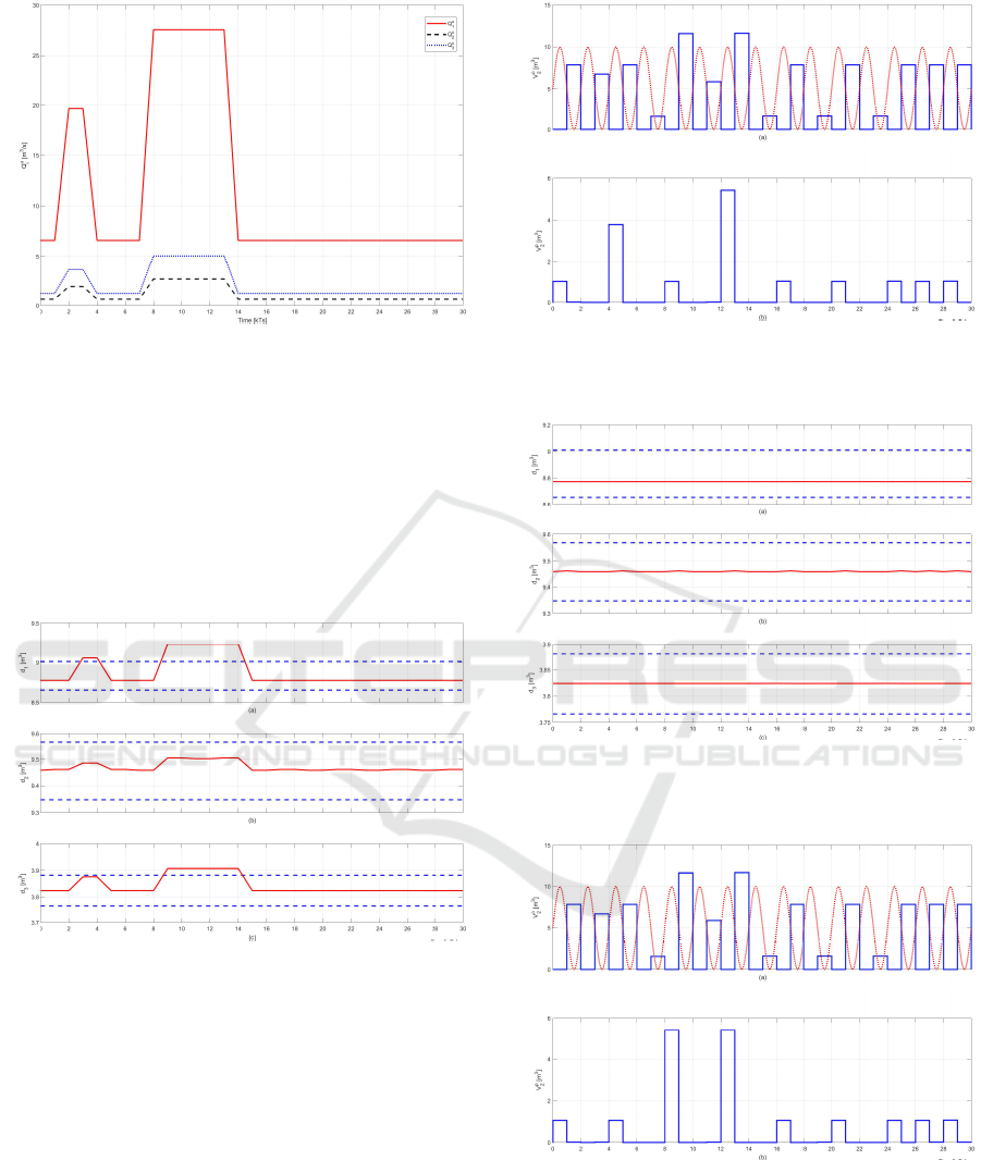
Figure 4: Uncontrolled discharges Q

, Q

and Q

for the

deﬁned scenario with two periods of strong rain, where a

sample time correspond to 6 hours.

sea only during low tide. The tide is depicted in red

dotted line in Figure 6.a. When additional water vo-

lumes that come from rain have to be rejected during

high tide, it is necessary to use the pump guaranteeing

the navigation condition in NR

(see sample times 4

and 12 in Figure 6.b). This strategy allows limiting

the cost due to the use of the pump.

Figure 5: Scenario 1: in red line, the water volume in (a)

the NR

, (b) the NR

and (c) the NR

, in blue dashed line

the allowed boundaries.

The second scenario (Scenario 2) is based on the

strong assumption that the water volumes from rainy

events are perfectly predicted. With this assumption,

the three NR keep perfectly their navigation objective

as it is depicted in Figure 7. In this case also, the

pump and the water rejection by gravity are used to

keep the objective in the NR

by taking into account

the tide (see Figure 8). The water volumes that are

pumped are not so different than the Scenario 1. In

this Scenario 2, the water volumes have been better

allocated between the three NR. This strategy allows

limiting the cost due to the use of the pump.

The third scenario (Scenario 3) consists in consi-

Figure 6: Scenario 1: water volumes that are rejected by (a)

gravity to the sea, (b) pump [m

], with the tide depicted in

red dotted line.

Figure 7: Scenario 2: in red line, the water volume in (a)

the NR

, (b) the NR

and (c) the NR

, in blue dashed line

the allowed boundaries.

Figure 8: Scenario 2: water volumes that are rejected by (a)

gravity to the sea, (b) pump [m

], with the tide depicted in

red dotted line.

dering an error of 30 % in the prediction of the water

volumes from rainy events. Based on this assumption,

the NR

is still the most impacted. However, its vo-

lume is kept inside the deﬁned boundaries (see Figure

ICINCO 2018 - 15th International Conference on Informatics in Control, Automation and Robotics

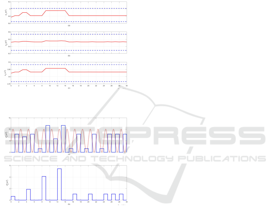
9.a). The objectives are guaranteed also for NR

and

as it is depicted in Figure 9.b and in Figure 9.c.

The pump and the water rejection by gravity are still

used to keep the objective in the NR

by taking into

account the tide (see Figure 8). The pumped volu-

mes are more progressive during the time, but not so

different from the two ﬁrst scenarios.

Figure 9: Scenario 3: in red line, the water volume in (a)

the NR

, (b) the NR

and (c) the NR

, in blue dashed line

the allowed boundaries.

Figure 10: Scenario 3: water volumes that are rejected by

(a) gravity to the sea, (b) pump [m

], with the tide depicted

in red dotted line.

The three scenarios show that the prediction of

strong rainy events is required to optimize the water

resource management of inland navigation networks.

However, the Scenario 3 indicates that the manage-

ment objectives can be kept even if a big error is made

on this prediction, i.e. an error of 30 %. Hence, a

strong effort have to be done on the design of accu-

rate predictive rainfall/runoff models.

5 CONCLUSIONS

In this paper, the integrated model and the ﬂow graph

that have been already proposed in past publications,

are adapted and improved to deal with the case of in-

land water systems with outlet to the sea. The water

allocation planning algorithm is also adapted to consi-

der these new elements. A realistic case study which

characteristics are based on the real inland waterways

of the north of France is presented to test these im-

proved tools and algorithm. The simulation results

show that the prediction of the impacts of rainy events

is necessary to guarantee the management objectives

even if an important error in prediction can be allo-

wed. Future works will be dedicated to improve the

predictive rainfall/runoff model. Then, the designed

tools and methods can be applied on a part of a real

inland waterway.

REFERENCES

Arkell, B. and Darch, G. (2006). Impact of climate change

on london’s transport network. Proceedings of the ICE

- Municipal Engineer, 159:231–237.

Bastin, G., Moens, L., and Dierick, P. (2009). Online ri-

ver ﬂow forecasting with hydromax : successes and

challenges after twelve years of experience. In pro-

ceedings of the 15th IFAC Symposium on System Iden-

tiﬁcation, Saint-Malo, France, July 6-8.

Bates, B., Kundzewicz, Z., Wu, S., and Palutikof, J. (2008).

Climate change and water. Technical repport, Inter-

governmental Panel on Climate Change, Geneva.

e, J., Terray, L., Martin, E., and Habetsi, F. (2009). Pro-

jected changes in components of the hydrological cy-

cle in french river basins during the 21st century. Wa-

ter Resources Research, 45.

Bourgin, F. (2014). Comment quantiﬁer lincertitude pr-

dictive en modlisation hydrologique ? : Travail explo-

ratoire sur un grand chantillon de bassins versants.

PhD thesis. Thse de doctorat dirige par Andrassian,

Vazken Hydrologie Paris, AgroParisTech 2014.

Brand, C., Tran, M., and Anable, J. (2012). The uk transport

carbon model: An integrated life cycle approach to

explore low carbon futures. Energy Policy, 41:107–

124.

Dakhlaoui, H., Ruelland, D., Tramblay, Y., and Barga-

oui, Z. (2017). Evaluating the robustness of concep-

tual rainfall-runoff models under climate variability

in northern tunisia. Journal of Hydrology, 550:201

– 217.

Ducharne, A., Habets, F., Pag

e, C., Sauquet, E., Viennot,

P., D

equ

e, M., Gascoin, S., Hachour, A., Martin, E.,

Oudin, L., Terray, L., and Thi

ery, D. (2010). Cli-

mate change impacts on water resources and hydro-

logical extremes in northern france. XVIII Conference

on Computational Methods in Water Resources, June,

Barcelona, Spain.

Water Asset Management Strategy based on Predictive Rainfall/Runoff Model to Optimize the Evacuation of Water to the Sea

Duviella, E. and Bako, L. (2012). Predictive black-box mo-

deling approaches for ﬂow forecasting of the liane ri-

ver. SYSID12, Bruxelles, Belgium, July 11-13.

Duviella, E., Nouasse, H., Doniec, A., and Chuquet, K.

(2016). Dynamic optimization approaches for re-

source allocation planning in inland navigation net-

works. ETFA2016, Berlin, Germany, September 6-9.

Duviella, E., Rajaoarisoa, L., Blesa, J., and Chuquet, K.

(2013). Adaptive and predictive control architecture

of inland navigation networks in a global change con-

text: application to the cuinchy-fontinettes reach. in

IFAC MIM conference, Saint Petersburg, 19-21 June.

Edijatno and Michel, C. (1989). Un mod

ele pluie-d

ebit

journalier

a trois param

etres. La Houille Blanche,

2:113 121.

Edijatno, Nascimento, N. D. O., Yang, X., Makhlouf, Z.,

and Michel, C.

EnviCom (2008). Climate change and navigation - water-

borne transport, ports and waterways: A review of cli-

mate change drivers, impacts, responses and mitiga-

tion. EnviCom - Task Group 3.

Ficchi, A. (2017). An adaptive hydrological model for mul-

tiple time-steps : diagnostics and improvements based

on ﬂuxes consistency. Theses, Universit

e Pierre et Ma-

rie Curie - Paris VI.

Horv

ath, K., Duviella, E., Rajaoarisoa, L., and Chuquet,

K. (2014a). Modelling of a navigation reach with

unknown inputs: the cuinchy-fontinettes case study.

Simhydro, Soﬁa Antipolis, 11-13 June.

Horv

ath, K., Duviella, E., Rajaoarisoa, L., Negenborn, R.,

and Chuquet, K. (2015a). Improvement of the naviga-

tion conditions using a model predictive control - the

cuinchy-fontinettes case study. International Confe-

rence on Computational Logistics, Delft, The Nether-

lands, 23-25 September.

Horv

ath, K., Petrecsky, M., Rajaoarisoa, L., Duviella, E.,

and Chuquet, K. (2014b). Mpc of water level in a navi-

gation canal - the cuinchy-fontinettes case study. Eu-

ropean Control Conference, Strasbourg, France, June

24-27.

Horv

ath, K., Rajaoarisoa, L., Duviella, E., Blesa, J., Pet-

reczky, M., and Chuquet, K. (2015b). Enhancing in-

land navigation by model predictive control of water

level the cuinchy-fontinettes case. Transport of Wa-

ter versus Transport over Water - Exploring the dyn-

amic interplay between transport and water - Carlos

Ocampo-Martinez, Rudy Engenborn (eds).

IWAC (2009). Climate change mitigation and adaptation.

implications for inland waterways in england and wa-

les. Report.

Jonkeren, O., Rietveld, P., and van Ommeren, J. (2007). Cli-

mate change and inland waterway transport: welfare

effects of low water levels on the river rhine. Journal

of Transport Economics and Policy, 41:387–412.

Kara, S., Sihn, W., Pascher, H., Ott, K., Stein, S., Schu-

macher, A., and Mascolo, G. (2015). A green and

economic future of inland waterway shipping. Proce-

dia CIRP - The 22nd CIRP Conference on Life Cycle

Engineering, 29:317 – 322.

Koetse, M. J. and Rietveld, P. (2009). The impact of cli-

mate change and weather on transport: An overview

of empirical ﬁndings. Transportation Research Part

D: Transport and Environment, 14(3):205 – 221.

Laurain, V. (2010). Contributions l’identiﬁcation de

mod

eeles param

etriques non lin

eaires. application la

modlisation de bassins versants ruraux. PhD thesis,

Universit

e Henri Poincar

e, Nancy 1.

Ljung, L. (1999). System identiﬁcation : theory for the user

(2nd Edition). Prentice Hall, Upper Saddle River.

Mallidis, I., Dekker, R., and Vlachos, D. (2012). The impact

of greening on supply chain design and cost: a case for

a developing region. Journal of Transport Geography,

22:118–128.

Mihic, S., Golusin, M., and Mihajlovic, M. (1993). Policy

and promotion of sustainable inland waterway trans-

port in europe - danube river. Renewable and Sustai-

nable Energy Reviews, 15:1801–1809.

Nash, J. E. and Sutcliffe, J. V. (1970). River ﬂow forecas-

ting through conceptual models part I: a discussion of

principles. Journal of Hydrology, 10(3):282–290.

Nouasse, H., Doniec, A., Lozenguez, G., Duviella, E., Chi-

ron, P., Archimde, B., and Chuquet, K. (2016a). Con-

straint satisfaction problem based on ﬂow transport

graph to study the resilience of inland navigation net-

works in a climate change context. IFAC Conference

MIM, Troyes, France, 28-30 June.

Nouasse, H., Horv

ath, K., Rajaoarisoa, L., Doniec, A., Du-

viella, E., and Chuquet, K. (2016b). Study of global

change impacts on the inland navigation management:

Application on the nord-pas de calais network. Trans-

port Research Arena, Varsovie, Poland.

Nouasse, H., Rajaoarisoa, L., Doniec, A., Chiron, P., Du-

viella, E., Archimde, B., and Chuquet, K. (2015).

Study of drought impact on inland navigation systems

based on a ﬂow network model. ICAT, Sarajevo, Bos-

nie Herzegovia.

Perrin, C., Michel, C., and Andr

eassian, V. (2003). Impro-

vement of a parsimonious model for streamﬂow simu-

lation. Journal of Hydrology, 279:275 – 289.

Previdi, F. and Lovera, M. (2009). Identiﬁcation of

parametrically-varying models for the rainfall-runoff

relationship in urban drainage networks. IFAC Pro-

ceedings Volumes, 42(10):1768 – 1773. 15th IFAC

Symposium on System Identiﬁcation.

Rajaoarisoa, L., Horv

ath, K., Duviella, E., and Chuquet, K.

(2014). Large-scale system control based on decen-

tralized design. application to cuinchy fontinette re-

ach. IFAC World Congress, Cape Town, South Africa,

24-29 August.

Segovia, P., Rajaoarisoa, L., Nejjari, F., Puig, V., and Du-

viella, E. (2017). Decentralized control of inland na-

vigation networks with distributaries: application to

navigation canals in the north of france. ACC17, Se-

attle, WA, USA, May 2426.

Siou, L. K. A., Johannet, A., Pistre, S., and Borrell, V.

(2010). Flash ﬂoods forecasting in a karstic basin

using neural networks: the case of the lez basin (south

of france). International Symposium on Karst ISKA,

ICINCO 2018 - 15th International Conference on Informatics in Control, Automation and Robotics

Malaga. In Advances in research in karst media. An-

dreo et al eds Springer.

oth, R., Felici, F., Heuberger, P. S. C., and den Hof, P.

M. J. V. (2007). Discrete time lpv i/o and state space

representations, differences of behavior and pitfalls of

interpolation. Proc. of the European Control Conf.,

Kos, Greece, July 5418 5425.

Wang, S., Kang, S., Zhang, L., and Li, F. (2007). Model-

ling hydrological response to different land-use and

climate change scenarios in the zamu river basin of

northwest china. Hydrological Processes, 22:2502–

2510.

Young, P. C. (1986). Time series methods and recursive

estimation in hydrological systems analysis. In River

ﬂow modelling and forecasting, D. A. Kraijenhoff, J.

R. Moll (eds). D. Reidel : Dordrecht, page 129 180.

Water Asset Management Strategy based on Predictive Rainfall/Runoff Model to Optimize the Evacuation of Water to the Sea