Nonlinear Adaptive Estimation by Kernel Least Mean Square with

Surprise Criterion and Parallel Hyperslab Projection along Afﬁne

Subspaces Algorithm

Angie Forero and Celso P. Bottura

School of Electrical and Computer Engineering, University of Campinas, Brazil

Keywords:

Adaptive Nonlinear Estimation, Machine Learning, Kernel Algorithms, Kernel Least Mean Square, Surprise

Criterion, Projection along Afﬁne Subspaces.

Abstract:

In this paper the algorithm KSCP (KLMS with Surprise Criterion and Parallel Hyperslab Projection Along

Afﬁne Subspaces) for adaptive estimation of nonlinear systems is proposed. It is based on the combination

of: - the reproducing kernel to deal with the high complexity of nonlinear systems; -the parallel hyperslab

projection along afﬁne subspace learning algorithm, to deal with adaptive nonlinear estimation problem; -

the kernel least mean square with surprise criterion that uses concepts of likelihood and bayesian inference

to predict the posterior distribution of data, guaranteeing an appropriate selection of data to the dictionary

at low computational cost, to deal with the exponential growth of the dictionary, as new data arrives. The

proposed algorithm offers high accuracy estimation and high velocity of computation, characteristics that are

very important in estimation and tracking online applications.

1 INTRODUCTION

Machine Learning algorithms for nonlinear estima-

tion have been widely exploited in the last years.

The supervised machine learning algorithms are ca-

pable of producing function approximations and sig-

nal predictions only from inputs and reference sig-

nals, using past information that has been learned and

different kinds of optimization and statistical techni-

ques. The high complexity of nonlinear systems

has represented a great challenge, but since the ap-

parition of the Mercer Kernel theorem (Aronszajn,

1950), the kernel properties have played an impor-

tant role in adaptive learning methods (Kivinen et al.,

2004), (Scholkopf and Smola, 2001), enabling the use

of well-developed linear techniques in nonlinear pro-

blems through the Reproducing Kernel Hilbert Space

(RKHS). Many methods have been proposed in the

area of kernel adaptive learning such as Kernel Le-

ast Mean Square (KLMS) (Liu et al., 2008), Kernel

Recursive Least Square (KRLS) (Engel et al., 2004),

Kernel Afﬁne Projection Algorithms (KAPA) (Sla-

vakis et al., 2008), Extended Kernel Recursive Least

Squares (EX-KRLS) (Haykin et al., 1997). Among

these methods the Afﬁne Projection Algorithm from

Ozeki and Umeda (Ozeki, 2016) a generalization

and improvement of the Normalized LMS algorithm,

is characterized by a low complexity like the Least

Mean Square (LMS) algorithm and has faster conver-

gence than the Normalized LMS algorithm. Howe-

ver, one of its disadvantage is that as more delayed

inputs are used its velocity decreases. Yukawa and

Takizawa (Takizawa and Yukawa, 2015) proposed a

more evolved version of Afﬁne Projection Methods

that uses ideas of projection-along-subspace and pa-

rallel projection to reduce the complexity and there-

fore increase the velocity of performance.

A well-known problem of kernel adaptive ﬁltering

methods is the exponential growth of the dictionary:

the set of past information learned and stored. As

new data arrives, incorporating the new data into the

dictionary requires an adequate policy to avoid un-

necessary calculations with an increasing number of

variables, which results in a problem of high com-

putational cost and low velocity performance, ma-

king these algorithms unsuitable for online applica-

tions. Many heuristic selection criteria for the dicti-

onary have been proposed like: Approximate Linear

Dependency (ALD) (Engel et al., 2004) and Novelty

Criterion (Platt, 1991). To solve this problem of dicti-

onary control we propose a solution based on the sur-

prise criterion of Liu (Liu et al., 2009a), as it offers

a solid mathematical criterion that evaluates the true

signiﬁcance of the new sample and if it will contribute

362

Forero, A. and Bottura, C.

Nonlinear Adaptive Estimation by Kernel Least Mean Square with Surprise Criterion and Parallel Hyperslab Projection along Afﬁne Subspaces Algorithm.

DOI: 10.5220/0006867803620368

In Proceedings of the 15th International Conference on Informatics in Control, Automation and Robotics (ICINCO 2018) - Volume 1, pages 362-368

ISBN: 978-989-758-321-6

to the learning system, deciding whether the new data

should be taken or discarded.

The surprise criterion calculates the probability of

the posterior distribution of data given the past infor-

mation learned, using log likelihood and Bayesian in-

ference to evaluate in a certain sense, how related or

known the new data can be for the learning system.

The surprise criterion for the conventional Kernel

afﬁne projection algorithm represents a high compu-

tational cost in the sense that it requires calculating

the inversion of the Gram matrix at every instant of

time, when only the calculation of the approximation

of the prediction variance is needed to decide whet-

her the new data are going to be inserted or not into

its dictionary. For this reason, we propose to use the

KLMS and the Surprise Criterion which have a low

computational cost (it will be shown in section 2.2.1),

in fact there are two different problems: 1) establish

with some mathematical criterion the dictionary con-

trol and 2) calculate the approximation of the nonli-

near function. We develop an algorithm which esta-

blishes the dictionary control based on ideas of the

KLMS-Surprise Criterion algorithm and approxima-

tes the nonlinear objective function based on ideas

of Parallel hyperslab projection along afﬁne subspace

algorithm, achieving with this, a method for adap-

tive nonlinear estimation with high velocity of per-

formance, high accuracy and low complexity. These

results will be shown through a computational expe-

riment and be compared with some other methods. In

section 2 the main ideas are discussed, in section 3 the

algorithm is presented, the computational experiment

is shown in section 4 and ﬁnally the conclusions are

presented in section 5.

2 MAIN IDEAS

2.1 Problem Deﬁnition and Notation

Consider the problem of adaptive estimation of a non-

linear system f , where the input data u ∈ U and the

signal reference d arrive at each instant of time.

To enable the use of the linear techniques, we deal

with the nonlinear estimation in the Reproducing Ker-

nel Hilbert Space (RKHS) where the inputs belong to

the domain U and are mapped into a high-dimensional

feature space F. The mapping will be done by the

nonlinear function ϕ(·), such that ϕ : U → F. Then,

with the transformed input ϕ(u), we are able to apply

a linear algorithm in order to obtain the estimate of

the nonlinear function.

Let ψ(·) be a real function of the Hilbert Space H ,

there exists a continuous, symmetric, positive-deﬁnite

function u

→k(u

) such that k : UxU → R associ-

ated with it; where k(·, u

) is the kernel function eva-

luated in u

, satisfying the reproducing property

ψ(u

) =< ψ(·),k(·,u

) >

(1)

From this property of the reproducing kernel and the

transformed input, we get:

k(u

) =< ϕ(u

),ϕ(u

) >

(2)

Due to this reproducing kernel property, it is possi-

ble to evaluate the kernel by using the inner product

operation in the feature space. As the algorithm is for-

mulated in terms of inner products, there is no need to

develop calculations in the high-dimensional feature

space, a great advantage of the kernel properties.

To obtain the best estimation ψ of the nonlinear

system f , a least squares approach for this nonlinear

regression problem, looks for the determination of a

function ψ(·) that minimizes the sum of squared er-

rors between the reference signals and the output es-

timator, given by

ψ(·) =

∑

i=1

k(·, u

) (3)

where h

is a coefﬁcient of k(·, u

) at time i.

2.2 Dictionary Control

Before calculating the optimal error solution to esti-

mate iteratively the nonlinear function f , we must de-

cide if the incoming data are signiﬁcant and therefore

they should be learned and inserted in the dictionary

or if they should be discarded by being insigniﬁcant.

For doing this we use as a rule for dictionary control

the Surprise Criterion of Liu (Liu et al., 2010), that

gives the uncertainty amount of the new data with re-

spect to the current knowledge of the learning system

and is deﬁned as follows: Surprise S

D(i)

is the nega-

tive log likelihood of the new data given the current

dictionary D

i+1

) = −log p(u

i+1

) (4)

where p(u

i+1

) is the posterior distribution of

i+1

In this sense, if the probability of occurrence of

i+1

} is large, it means that the new data

are known by the learning system and therefore there

is no need to be learned; in the other case, if the proba-

bility is small, it means that the new data are unknown

by the learning system and they should be learned or

they are ”abnormal”, which indicates that they can

come from the errors or perturbations.

By using Bayesian inference and assuming all the in-

puts with a normal distribution, the posterior probabi-

lity density p(u

i+1

can be evaluated by

Nonlinear Adaptive Estimation by Kernel Least Mean Square with Surprise Criterion and Parallel Hyperslab Projection along Afﬁne

Subspaces Algorithm

363

p(u

i+1

) = p(d

i+1

)p(u

i+1

)

√

2πσ

i+1

exp

−

i+1

−

i+1

)

2σ

i+1

p(u

i+1

)

(5)

and

i+1

= −log[p(u

i+1

)]

= log

√

2π + log σ

i+1

−

i+1

)

2σ

i+1

−log[p(u

i+1

)]

(6)

Assuming that the distribution p(u

i+1

) is uniform, the

equation (6) can be simpliﬁed to

i+1

= log σ

i+1

−

i+1

)

2σ

i+1

(7)

From the equation above, we can observe that the cal-

culation of the surprise can be deduced directly from

the variance σ

i+1

and the error e = (d

i+1

−

i+1

2.2.1 Kernel Least Mean Square with Surprise

Criterion (KLMS-SC)

For kernel adaptive ﬁltering, the KLMS algorithm of-

fers a great advantage in terms of simplicity. The

calculation of the prediction variance is simpliﬁed by

using a distance measure M, an approximation that

selects the nearest inputs in the dictionary to estimate

the total distance and deﬁned as:

M = min

∀b∀c

∈D

kϕ(u

i+1

) −bϕ(c

)k (8)

where c

is an element of the dictionary and b is a

coefﬁcient. Solving the equation 8 we get

i+1

= λ+k(u

i+1

)−max

∀c

∈D

i+1

)

k(c

)

(9)

where v

i+1

denotes the prediction variance and λ is a

regularization parameter. For more details of KLMS-

Surprise Criterion see (Liu et al., 2010).

In contrast, if the Kernel Afﬁne Projection Algo-

rithm with surprise criterion were used, we should

solve the following problem:

M = min

∀b∀n

∈D

kϕ(u

i+1

) −

∑

j=1

ϕ(n

)k (10)

that results in

i+1

= λ + k(u

i+1

) −h

+ λI]

−1

(11)

where h

= [k(u

i+1

),...,k(u

i+1

)]

, I is the

identity matrix and G

is the Gram matrix.

From the equation above, we see that the calcu-

lation of the prediction variance includes the inver-

sion of the Gram matrix G for each instant of time.

This is very computationally expensive and is not al-

ways possible to calculate the inversion of the Gram

Matrix. However, we only need to calculate the pre-

diction variance and the prediction error of the new

data with respect to the learned system, to decide if

the new data are going to be inserted to the dictionary

or not. This is independent of the calculation process

of the approximation of the gradient direction and

of the estimation of the nonlinear objective function.

For this reason we are able to establish one method

for selection of data (dictionary control) and another

method for the nonlinear function estimation, and we

can take the advantage of the versatility of the Af-

ﬁne Projection Algorithms. Thus, we propose an al-

gorithm that uses the KLMS and the Surprise Crite-

rion for dictionary control and the parallel hyperslab

projection along afﬁne subspace for gradient direction

calculation that we call KSCP.

2.3 Parallel Hyperslab Projection along

Afﬁne Subspace (φ-PASS)

Let ψ

i+1

be the next estimate of the current estimate

obtained by its afﬁne projection onto a hyperplane

of optimal solutions Π

deﬁned by

:= {ψ;d

−hψ,k(·,u

)i = 0} (12)

We suppose that ψ

belongs to the dictionary D

for estimation updating. As it is possible that ψ

/∈ D

for the dictionary control, the solution we adopt is

the parallel hyperslab projection along afﬁne sub-

space (φ-PASS) by Takizawa and Yukawa (Takizawa

and Yukawa, 2013). It is based on projection-along-

subspace, where the intersection of the dictionary

space D

with the hyperplane Π

is calculated and the

current estimate ψ

is projected onto the intersection

∩Π

, that is equivalent to the projection of ψ

onto

along D

Thus, once the KLMS with surprise criterion al-

gorithm has established that the new data should be

learned, the estimate of the nonlinear function is cal-

culated using the Φ-PASS, enabling in all cases that

the estimate be updateable. Another advantage of

the Φ-PASS algorithm is the idea of parallel projecti-

ons, where using the p most recent measurements

)

l∈L

, (where L

:= (i,i −1, ..., i − p + 1) is the

index set of data) at each time and accommodating

into the hyperplanes Π

l∈L

, the current estimate ψ

is projected onto these hyperplanes in parallel, and

the direction of the next estimate is obtained in the

average point of the projections. This approach im-

proves the velocity of convergence and the noise ro-

bustness.

ICINCO 2018 - 15th International Conference on Informatics in Control, Automation and Robotics

364

3 THE KSCP ALGORITHM

The proposed algorithm KSCP (KLMS with Surprise

Criterion and Parallel Hyperslab Projection along Af-

ﬁne Subspace) ﬁrst establishes a dictionary control

which guarantees that only the signiﬁcant data are

going to be used for the estimation, allowing an ap-

propriate use of resources to avoid the unnecessary

calculations with redundant data or data from errors

or perturbations, improving the calculation velocity of

the algorithm at low computational cost using ideas of

kernel least mean square. This characteristic is very

important in online applications. For calculating the

gradient direction and the approximation of the non-

linear function at each instant of time in the adaptive

way, we use the projection along afﬁne subspace and

parallel projection approaches, achieving high accu-

racy and fast convergence.

The algorithm works in the following way:

When {u

i+1

} arrives, the inputs are transfor-

med using the kernel Gaussian function:

k(u

) = exp(−γku

−u

) (13)

wherewith we can use the afﬁne projection technique

into the transformed inputs for the treatment of the

nonlinear system.

With the result of the kernel evaluation in (13),

construct

i+1

= [k(u

i+1

),··· ,k(u

i+1

)]

(14)

where c

is a dictionary element at time i.

The output is calculated using the estimative ψ

obtained by the parallel hyperslab projection along af-

ﬁne subspace. It should be noted that if the dictionary

control establishes that the data should not be learned,

there is no need to update the estimative and the last

calculated value of the estimative will be taken. The

output is obtained by

i+1

) = x

i+1

(15)

initialized with ψ

= 0.

The prediction error is calculated by

i+1

= d

i+1

−

i+1

) (16)

The prediction variance is calculated using the Kernel

least mean squares approach

i+1

= λ + k(u

i+1

) −max

∀c

∈D

i+1

)

k(c

)

(17)

which offers a great advantage due to its simplicity,

with no need to compute the Gram matrix inversion

in the control dictionary step. It avoids the high com-

putational costs for achieving fast performance.

With the predictions of variance and error, we cal-

culate the Surprise Criterion by

i+1

log v

i+1

(18)

Based on the Surprise Criterion we establish the fol-

lowing rule for dictionary control:

• S

i+1

> T

⇒ Abnormal and Discarded

• T

≥ S

i+1

≥ T

⇒ Learnable

• S

i+1

< T

⇒ Redundant and Discarded

the abnormality threshold and T

the redundancy

threshold, are parameters dependent of the problem.

It is possible to make a trade-off between more accu-

racy or more velocity of performance by adjusting the

parameters T

and T

If the new data are learnable, they will be inserted

in the dictionary D

and the expansion coefﬁcient ψ

will be calculated and updated. If not the system just

takes the last estimate and returns to the beginning for

waiting new data.

With this step we avoid the waste of resources as

any aditional calculation would be done on insigni-

ﬁcant data. This helps the algorithm to be more ef-

fective. It also improves the execution of the approxi-

mation of the gradient direction because this approxi-

mation involves calculations with matrices that grows

exponentially with the dictionary. With this approach

we get a dictionary that uses only the essential quan-

tity of data.

If the data are learnable and inserted in the dicti-

onary we are going to project the current estimate ψ

onto the closed convex set deﬁned by

(i)

:= V

(i)

∩Π

⊂ D

(19)

where V is an afﬁne subspace of the dictionary deﬁ-

ned by

:= span (k(·,u

))

j∈J

(i)

+ ψ

⊂ D

(20)

and (k(. , u

))

j∈J

(i)

is the set of selected elements.

Then, the projection of ψ onto the convex set is

given by

ψ = ψ + βP

k(·, u) (21)

where β is calculated by

β = ς

max(| d −ψ(u) |, 0)

∑

j∈J

k(u, u

)

(22)

with the signum function ζ(·) and

k(·, u) =

∑

j∈J

k(u, u

) (23)

Nonlinear Adaptive Estimation by Kernel Least Mean Square with Surprise Criterion and Parallel Hyperslab Projection along Afﬁne

Subspaces Algorithm

365

The projection P

k(·, u) is obtained solving the

normal equation:

α = G

−1

y (24)

where G is the Gram matrix

G =







k(u

) k(u

) ··· k(u

)

k(u

) k(u

) ··· k(u

)

k(u

) k(u

) ··· k(u

)







(25)

and

y :=



k(u, u

) k(u, u

) ··· k(u,u

)



(26)

Finally the nonlinear estimate is calculated by

i+1

= ψ

+ λ

∑

l∈L

−ψ

(27)

with w

≥ 0 and ψ

is updated in equation (15)

4 COMPUTATIONAL

EXPERIMENT

In this section we show the performance of the propo-

sed algorithm KSCP and compare it with some met-

hods: Kernel Afﬁne Projection with Coherence Cri-

terion (KAP) (Richard et al., 2009), (Said

e et al.,

2012) Kernel Least Mean Square with Coherence-

Sparsiﬁcation criterion and Adaptive L1-norm regu-

larization (KLMS-CSAL1) (Gao et al., 2013) and

Extended Recursive Least Squares (EXKRLS) (Liu

et al., 2009b). For these algorithms we used the tool-

box Kafbox (Van Vaerenbergh and Santamar

ıa, 2013)

We employ the benchmark sinc function estima-

tion which is often used for nonlinear regression ap-

plications. The synthetic data are generated by

= sinc(x

) + ν

(28)

where

sinc(x) =



sin(x)/x x 6= 0

1 x = 0

(29)

is a zero-mean Gaussian noise with variance 0.04.

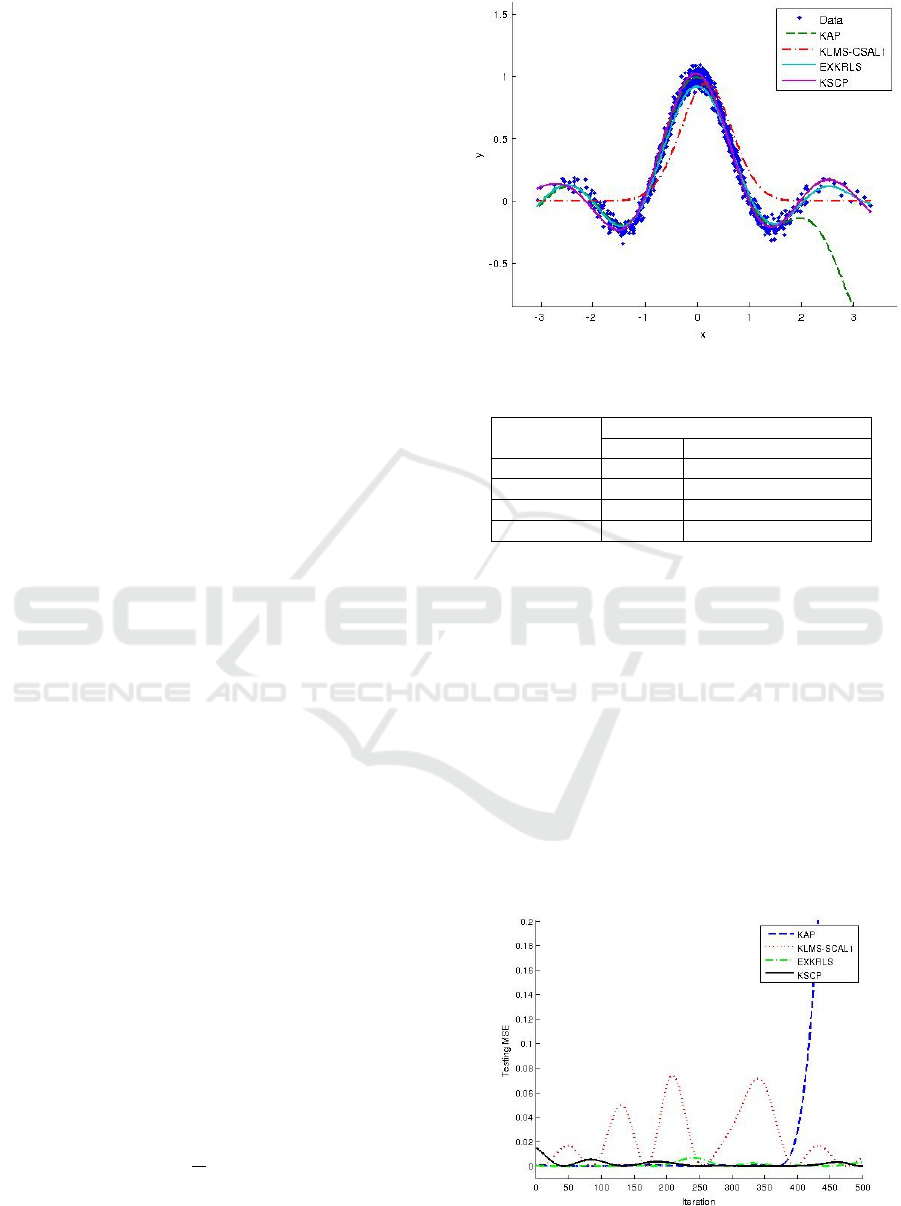
In the simulation we use 1000 samples for trai-

ning and 500 samples for testing. The estimation re-

sults are showed in Fig. 1 and in Table. 1 where the

mean square error (MSE) for the estimation for each

method is presented. The MSE is calculated by

MSE =

∑

i=1

− ˆy

)

(30)

where y

is the reference or desired value and ˆy

is the

estimated value.

Figure 1: Sinc Function Estimation.

Table 1: Performance of the Algorithms.

Algorithm Performance

MSE (dB) Time of Execution (seconds)

KAP -10.33 0.31

KLMS-CSAL1 -16.48 0.27

EXKRLS -29.34 0.88

KSCP -32.42 0.72

The learning curve of each algorithm is presented

in Fig. 2. The parameters setting used by each one

of the methods are the following: for KAP the cohe-

rence criterion µ

= 0.95, the step size η = 0.5, the re-

gularization term λ = 0.01, and the kernel parameter

γ = 1;for KLMS-CSAL1 the coherence criterion µ

0.95, the step size η = 0.1, the sparsiﬁcation thres-

hold ρ = 5x10

−4

, and the kernel parameter γ = 0.5;

for EXKRLS the state forgetting factor α = 0.99, the

data forgetting factor β = 0.99, the regularization fac-

tor λ = 0.01, the trade-off between modeling variation

and measurement disturbance q = 1x10

−3

and the ker-

nel parameter γ = 1; for KSCP the abnormality thres-

hold T

= 1, the redundancy threshold T

= −0.5, the

step size η = 0.5, the regularization term λ = 0.01,

Figure 2: Learning Curve for KAPCC, KLMS-CSAL1 and

KSCP.

ICINCO 2018 - 15th International Conference on Informatics in Control, Automation and Robotics

366

number of hyperslabs p = 8, the weight coefﬁcient

ω = 0.1250 and the kernel parameter γ = 1.

The obtained results lead to the following obser-

vations:

• The four algorithms presented in this experiment

have a fast performance, taking less than 1 minute

in the estimation with 1000 training samples. As

is showed in Table I, the KSCP achieves the mini-

mum mean square error, the KAP and the KLMS-

SCAL1 achieves more velocity in execution but

with a higher mean square error. It is important

to highlight that the settings of the T

and T

pa-

rameters are essential for the execution time and

the accuracy. The abnormality threshold parame-

ter T

can be adjusted for achieving more velocity

and the redundancy threshold parameter T

must

be adequately limited to guarantee high accuracy.

• The learning curve ﬁgure showed that in the Ker-

nel Afﬁne Projection algorithm, the mean square

error begins to grow exponentially in the iteration

number 400; the KLMS-SCAL1 takes several ite-

rations to stabilize and the EXKRLS and KSCP

reach zero and remain stable from the ﬁrst 50 ite-

rations for the considered situation.

5 CONCLUSIONS

This paper presents our proposed algorithm KSCP

for adaptive nonlinear estimation. The KSCP impro-

ves the estimation performance based on 3 aspects:

First, an effective dictionary control is established,

guaranteeing an exhaustive selection of the most im-

portant data for the estimation, and low computational

complexity, basing not on heuristics but on a strong

mathematical foundation approach with statistical and

probabilistic techniques. Second, we take advantage

of the Kernel Least Mean Square and the Surprise Cri-

terion combining them to reduce the complexity of

the calculations of variance prediction and error pre-

diction of the incoming data. Third, for the high accu-

racy goal, we use the Parallel Hyperslab Projection

Along Afﬁne Subspace.

With all of these ideas, we achieve a fast conver-

gence, high accuracy, small size of dictionary and fast

performance algorithm, which is demonstrated by the

computational experiment and the comparison with

some important and recognized algorithms like Ker-

nel Afﬁne Projection with Coherence Criterion, Ker-

nel Least Mean Square with Coherence-Sparsiﬁcation

criterion and Adaptive L1-norm regularization and

Extended Recursive Least Squares.

REFERENCES

Aronszajn, N. (1950). Theory of reproducing kernels.

Transactions of the American mathematical society,

68(3):337–404.

Engel, Y., Mannor, S., and Meir, R. (2004). The kernel

recursive least-squares algorithm. IEEE Transactions

on Signal Processing, 52(8):2275–2285.

Gao, W., Chen, J., Richard, C., Huang, J., and Flamary, R.

(2013). Kernel lms algorithm with forward-backward

splitting for dictionary learning. In 2013 IEEE Inter-

national Conference on Acoustics, Speech and Signal

Processing, pages 5735–5739.

Haykin, S., Sayed, A. H., Zeidler, J. R., Yee, P., and Wei,

P. C. (1997). Adaptive tracking of linear time-variant

systems by extended rls algorithms. IEEE Transacti-

ons on Signal Processing, 45(5):1118–1128.

Kivinen, J., Smola, A. J., and Williamson, R. C. (2004).

Online learning with kernels. IEEE Transactions on

Signal Processing, 52(8):2165–2176.

Liu, W., Park, I., and Principe, J. C. (2009a). An infor-

mation theoretic approach of designing sparse kernel

adaptive ﬁlters. IEEE Transactions on Neural Net-

works, 20(12):1950–1961.

Liu, W., Park, I., Wang, Y., and Principe, J. C. (2009b). Ex-

tended kernel recursive least squares algorithm. IEEE

Transactions on Signal Processing, 57(10):3801–

3814.

Liu, W., Pokharel, P. P., and Principe, J. C. (2008). The ker-

nel least-mean-square algorithm. IEEE Transactions

on Signal Processing, 56(2):543–554.

Liu, W., Principe, J., and Haykin, S. (2010). Kernel Adap-

tive Filtering: A comprehensive Introduction. Wiley,

1 edition.

Ozeki, K. (2016). Theory of afﬁne projection algorithms for

adaptive ﬁltering. Springer.

Platt, J. (1991). A resource-allocating network for function

interpolation. Neural computation, 3(2):213–225.

Richard, C., Bermudez, J. C. M., and Honeine, P. (2009).

Online prediction of time series data with kernels.

IEEE Transactions on Signal Processing, 57(3):1058–

1067.

Said

e, C., Lengell

e, R., Honeine, P., Richard, C., and Ach-

kar, R. (2012). Dictionary adaptation for online pre-

diction of time series data with kernels. In 2012 IEEE

Statistical Signal Processing Workshop (SSP), pages

604–607.

Scholkopf, B. and Smola, A. (2001). Learning with Kernels.

Cambridge. MIT Press, 1 edition.

Slavakis, K., Theodoridis, S., and Yamada, I. (2008). On-

line kernel-based classiﬁcation using adaptive pro-

jection algorithms. IEEE Transactions on Signal Pro-

cessing, 56(7):2781–2796.

Takizawa, M. and Yukawa, M. (2013). An efﬁcient data-

reusing kernel adaptive ﬁltering algorithm based on

parallel hyperslab projection along afﬁne subspaces.

In 2013 IEEE International Conference on Acoustics,

Speech and Signal Processing, pages 3557–3561.

Nonlinear Adaptive Estimation by Kernel Least Mean Square with Surprise Criterion and Parallel Hyperslab Projection along Afﬁne

Subspaces Algorithm

367

Takizawa, M. and Yukawa, M. (2015). Adaptive non-

linear estimation based on parallel projection al-

ong afﬁne subspaces in reproducing kernel hilbert

space. IEEE Transactions on Signal Processing,

63(16):4257–4269.

Van Vaerenbergh, S. and Santamar

ıa, I. (2013). A compa-

rative study of kernel adaptive ﬁltering algorithms. In

2013 IEEE Digital Signal Processing (DSP) Works-

hop and IEEE Signal Processing Education (SPE).

ICINCO 2018 - 15th International Conference on Informatics in Control, Automation and Robotics

368