
Conical Tank Level Supervision using a Fractional Order Model
Reference Adaptive Control Strategy
Hanane Balaska
1
, Samir Ladaci
2
and Youcef Zennir
3
1
Department of Science and Technology, University Larbi Ben Mhidi, Oum El-Bouaghi, 04000, Algeria
2
Department of E.E.A., National Polytechnic School of Constantine, BP 75 A, Nouvelle ville Ali Mendjli,
25100 Constantine, Algeria
3
Department of Petrochemistry, University of Skikda, Route d’Elhadaiek, BP 26, Skikda 21000, Algeria
Keywords:
Model Reference Adaptive Control, Fractional Order System, Fractional Integration, Direct Auto Adjustable
Control, Non Linear System, Robustness, Parametric Variation.
Abstract:
This paper proposes a fractional order model reference adaptive control (FO-MRAC) design in order to com-
mand the level of a conical tank system. The FO-MRAC is based on the choice of a fractional reference model
which specifies the closed loop desired performances. Also, the control strategy adopted introduces fractional
integration in the phase of corrector parameters updating. Model reference adaptive controller of integer or-
der and of fractional order are applied to the non linear system and compared. From the simulation results,
we concluded that FO-MRAC is the controller presenting the best performances, and especially in case of
measurements noise, and parametric variations.
1 INTRODUCTION
Fractional order systems are attracting more and more
researchers in different domains of science and engi-
neering (Mathieu et al., 2003; Ma et al., 2009; El-
sayed and Gaafar, 2003). Fractional order control is a
generalization of the classic control theory of integer
order, its major interest is to improve the control sys-
tem performances using the concepts of non-integer
derivation and fractional order systems. Dynamic
Systems and Fractional Order Controllers, which are
based on the fractional calculation, have gathered the
attention of several researchers. The most known
fractional order control structures are: CRONE con-
troller (Outsaloup, 1991), Fractional PI
λ
D
µ
controller
(Podlubny, 1999), and fractional adaptive control
(Ladaci et al., 2008).
Adaptive control is one of the popular control tech-
niques applied in industrial applications. This com-
mand consists in adapting the regulator on line with
the variations of the regulated process to ensure a
constant quality of performances. The main reason
which have encouraged researchers to move toward
fractional order adaptive control and essentially to
the fractional order model reference adaptive control
(FO-MRAC) is that The MRAC command is based
on the choice of a reference model that specifies the
desired performances in closed loop, and many re-
search works proved the very good performances of
fractional systems relatively to those of integer order
(Outsaloup, 1995; Ladaci and Bensafia, 2016).
Many fractional order control structure based on
MRAC have been developed in literature (Ladaci and
Charef, 2012). An indirect model reference adaptive
control is used to control a class of fractional order
systems was introduced in (Chen et al., 2016). In
(Vinagre et al., 2002; Ladaci and Charef, 2003), the
authors investigated the use of fractional order pa-
rameter adjustment rule and the employment of frac-
tional order reference model. The use of a fractional
model and the introduction of fractional derivative fil-
ter at the plant output was introduced in (Ladaci and
Charef, 2006).
In this paper, we propose to control a nonlinear
dynamical plant with fractional order model refer-
ence adaptive control to improve the system perfor-
mances. We will deal with the problem of conical
tank level control, which has been widely studied and
several control techniques have been employed, even
with model predictive control (Warier and Venkatesh,
2012) and fractional order PI
λ
D
µ
controllers(Jauregui
et al., 2016).
This work is organized as follows: Section 2 presents
some theoretical concepts on fractional order systems.
214
Balaska, H., Ladaci, S. and Zennir, Y.
Conical Tank Level Supervision using a Fractional Order Model Reference Adaptive Control Strategy.
DOI: 10.5220/0006869602140221
In Proceedings of the 15th International Conference on Informatics in Control, Automation and Robotics (ICINCO 2018) - Volume 1, pages 214-221
ISBN: 978-989-758-321-6
Copyright © 2018 by SCITEPRESS – Science and Technology Publications, Lda. All rights reserved

The proposed FMRAC strategy is presented in Sec-
tion 3, and the conical tank modelization is given in
Section 4. Section 5 shows the simulation results.
Section 6 is dedicated to the main conclusions and
future researches.
2 FRACTIONAL ORDER
SYSTEMS
Fractional calculus is the domain of analytical math-
ematics which deals with the study and application of
arbitrary order of integrals and derivatives.
2.1 Definitions
The commonly used definitions of the fractional or-
der integrals and derivative are the Riemann-Liouville
(R-L) and Gr¨unwald-Letnikov(G-L) definitions (Old-
ham and Spanier, 1974; Bourouba et al., 2018).
The R-L fractional order integral of order λ > 0 is de-
fined as:
I
λ
RL
g(t) = D
−λ
RL
g(t) (1)
=
1
Γ(λ)
Z
t
0
(t −τ)
λ−1
g(τ)d(τ)
and the expression of the R-L fractional order deriva-
tive of order µ > 0 is:
D
µ
g(t) = D
m
D
−ν
g(t)
, µ > 0, (2)
where Γ(.) is the Euler’sgamma function and the inte-
ger m is such that (m−1) < µ < m and ν = m−µ > 0.
The GL fractional order integral of order λ > 0 is
given by:
I
λ
GL
g(t) = D
−λ
GL
g(t) (3)
= lim
h→0
k
∑
j=0
(−1)
j
−λ
j
g(kh − jh)
Where h is the sampling period and the coefficients
and ω
(−λ)
0
=
−λ
0
the coefficients of the following
binomial:
(1−z)
−λ
=
∞
∑
j=0
ω
(−λ)
j
z
j
(4)
The GL fractional order derivative of order µ > 0
is also given by
D
µ
GL
g(t) =
d
µ
dt
µ
g(t) (5)
= lim
h→0
h
−µ
k
∑
j=0
(−1)
j
µ
j
g(kh − jh)
where h is the sampling period and the coefficients
ω
(µ)
j
=
µ
j
=
Γ(µ+1)
Γ( j+1)Γ(µ−j+1)
,
with ω
(µ)
0
=
µ
0
= 1,
are those of the polynomial:
(1−z)
µ
=
∞
∑
j=0
(−1)
j
µ
j
z
j
=
∞
∑
j=0
ω
(µ)
j
z
j
(6)
2.2 Linear Approximation of Fractional
Order Transfer Functions
For the purpose of our approach we need to use an in-
teger order model approximation of the fractional or-
der model reference in order to implement the adapta-
tion algorithm. For this aim, we use the so-called sin-
gularity function method proposed by (Charef et al.,
1992), and precisely for fractional first order system
of the form:
H(s) =
1
(1+ s p
T
)
β
(7)
with β a positive real number such that 0 < β < 1.
The approximation is given by:
H(s) ≈
∏
L−1
v=0
1+
s
z
v
∏
L
v=0
1+
s
p
v
(8)
Where the singularities are given by:
p
v
= (ab)
v
p
0
v = 1,2, 3,..., L−1
z
v
= (ab)
v
ap
0
v = 1,2, 3,..., L−1
(9)
with,
p
0
= p
T
10
ε
20β
(10)
a = 10
ε
10(1−β)
b = 10
ε
10β
β =
log(a)
log(ab)
ε is the tolerated error in dβ. L + 1 is the total num-
ber of singularities that can be determined by the fre-
quency band of the system.
2.3 Numerical Approximation of
Riemann Fractional Integral
In our work, we need to use a numerical approxima-
tion for the analytical formulas of the fractional order
Conical Tank Level Supervision using a Fractional Order Model Reference Adaptive Control Strategy
215

Process
Adjustment
mechanism
Reference
Model
Controller
u
y
u
c
y
m
Figure 1: Block Diagram for MRAC approach.
operator and more precisely for the integral of Rie-
mann introduced in (Ladaci and Charef, 2006):
Putting:
t = k∆
Where t is the current time, k an integer, and ∆ sam-
pling period. We obtain:
I
λ
g(k∆) =
∆
Γ(λ)
k−1
∑
τ=0
(k∆ −τ∆)
λ−1
g(τ∆) (11)
=
∆
λ
Γ(λ)
k−1
∑
τ=0
(k−τ)
λ−1
g(τ∆)
3 FRACTIONAL ORDER MODEL
REFERENCE ADAPTIVE
CONTROL
3.1 Model Reference Adaptive Control
It’s one of the most used adaptive control approaches,
in which the desired performances are specified by the
choice of a reference model.
A block diagram representing the principle of this ap-
proach is given in the figure 1.
The reference model adaptive control system has
an ordinary feedback loop composed of the process
and the regulator and another feedback loop which al-
lows the change of the regulator parameters.
We consider a single input single output system
(SISO) described by the equation:
Ay(t) = Bu(t) (12)
Where u is the control signal and y is the output signal.
A and B represent polynomials functions of either the
differential operator p = d/dt, or the shift operator in
advance q.
The desired closed-loop response is specified by the
reference model output y
m
.
A
m
y
m
(t) = B
m
u
r
(t) (13)
A general linear regulator can be described by:
Ru(t) = Tu
r
(t) −Sy(t) (14)
where R, S, and T are polynomials. And we get the
closed-loop system:
y(t) =
BT
AR+ BS
u
r
(t) (15)
The mechanism of adjustment of the regulator param-
eters can be obtained using the law of MIT, which is
the original approach for the MRAC.
To represent the MIT law, we consider a closed-loop
system in which the regulator has a vector θ of ad-
justable parameters. Let e be the error between the
output y of the closed loop and that of the reference
model y
m
. The adjustment of the parameters is done
in such a way as to minimize a cost function defined
by
J(θ) =
1
2
e
2
(16)
To minimize J, we have to change the parameters in
the direction of the negative gradient of J, and we
have the famous MIT law:
dθ
dt
= −γ
δJ
δθ
= γϕe (17)
ϕ = −
δe
δθ
, and γ is the adaptation gain.
The following standardized algorithm is less sensitive
to signal levels:
dθ
dt
= γ
ϕe
α+ ϕ
T
ϕ
(18)
The control signal is computed using the following
relation:
u = ϕ
T
θ (19)
Where, ϕ is the regression vector containing the mea-
sured input and output signals u and y and the input
reference signal u
r
.
3.2 Fractional approach
In this work we will consider a fractional order refer-
ence model which will be implemented using the sin-
gularity approximation method proposed by (Charef
et al., 1992). Also, in the phase of updating the pa-
rameters of the corrector, we will use the fractional
order parameter adaptation law proposed in (Ladaci
and Charef, 2006) instead of equation (18) given by:
d
m
θ
dt
m
= γ
ϕe
α+ ϕ
T
ϕ
(20)
And we will use the numerical Riemann approxima-
tion (11) to obtain fractional order integral of the re-
lation (20).
ICINCO 2018 - 15th International Conference on Informatics in Control, Automation and Robotics
216
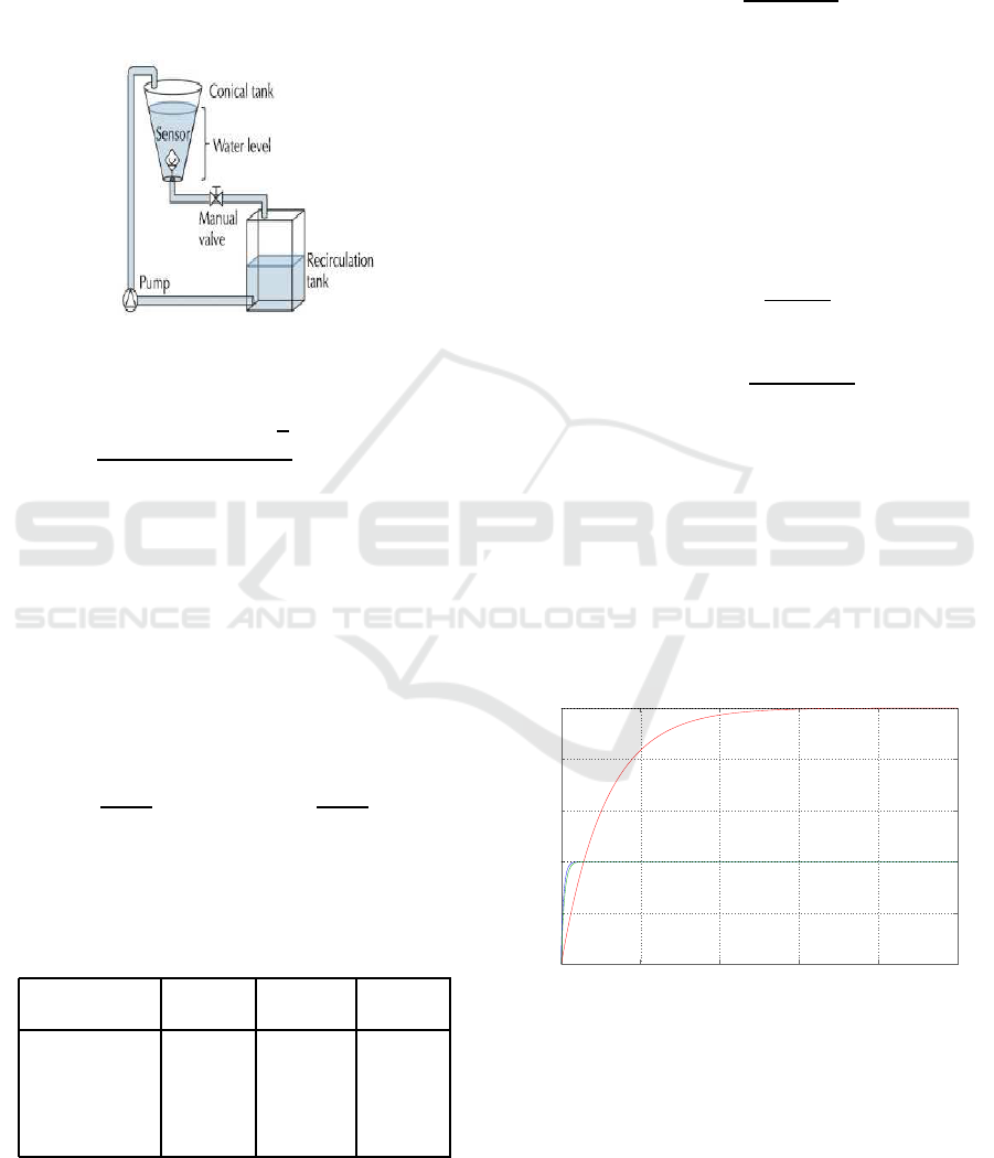
4 CONICAL TANK SYSTEM
The layout of the conical tank system is shown in Fig-
ure 2. The water is pumped from the bottom of the
recirculating tank to the upper part of the conical tank
by means of a pump driven by an induction motor of
variable speed driven by a variable frequency drive.
From (Jauregui et al., 2016), the nonlinear model for
Figure 2: Conical tank configuration.
the conical tank is represented by the following equa-
tion:
˙
h =
5.43f −78.23 + µ
√
h
0.65h
2
+ 11.4h + 17.1
= g(h, f) (21)
With µ = −20.63, f is the input and represent the
electrical network frequency expressed in % as a per-
centage of the nominal frequency (50Hz) and ranges
in the interval 0%−100%, h is the output and repre-
sent the water level inside the conical tank expressed
in cm, g(h, f) is a non linear function of these two
variables showing clearly the nonlinearities of the
conical tank system.
The system is linearized around 3 operating points
(h
op
, f
op
). These approximations are given by:
˙
h = W(h−h
op
) + Z( f − f
op
) (22)
With W =
δg(h, f)
δh
(h
op
, f
op
)
and Z =
δg(h, f)
δf
(h
op
, f
op
)
.
To determine the operating points the whole operation
range 15cm−60cm is divided into three segments, as
illustrated in Table 1.
Table 1: Operating points and parameters of linearized
models.
Low Medium High
level level level
Interval (cm) 15-30 30-45 45-60
h
op
(cm) 22.5 37.5 52.5
f
op
(%) 32.42 37.66 41.92
W -0.0036 -0.0012 -0.0006
Z 0.009 0.004 0.0022
In our work, we try to control the nonlinear sys-
tem around only one operation point (Low level).
So, the linearized system is represented by equation
(22), with W = −0.0036, and Z = 0.009, By posing:
y(t) = h −hop, and u(t) = f − fop, we obtain the
following transfer function (Deghboudj and Ladaci,
2017):
G(s) =
0.009
s+ 0.0036
(23)
5 SIMULATION RESULTS
In this Section, we will apply the proposed fractional
order adaptive control technique to the tank level
control, with the transfer function given in equation
(23).Let us chose reference model transfer functions
of integer order and fractional order respectively:
G
m
(s) =
1
1+ 20s
(24)
and
G
mf
(s) =
1
(1+ 20s)
0.6
(25)
G
mf
is approximated to an integer order model using
the singularity function method (Charef et al., 1992).
The sampling period is ∆ = 0.1sec.
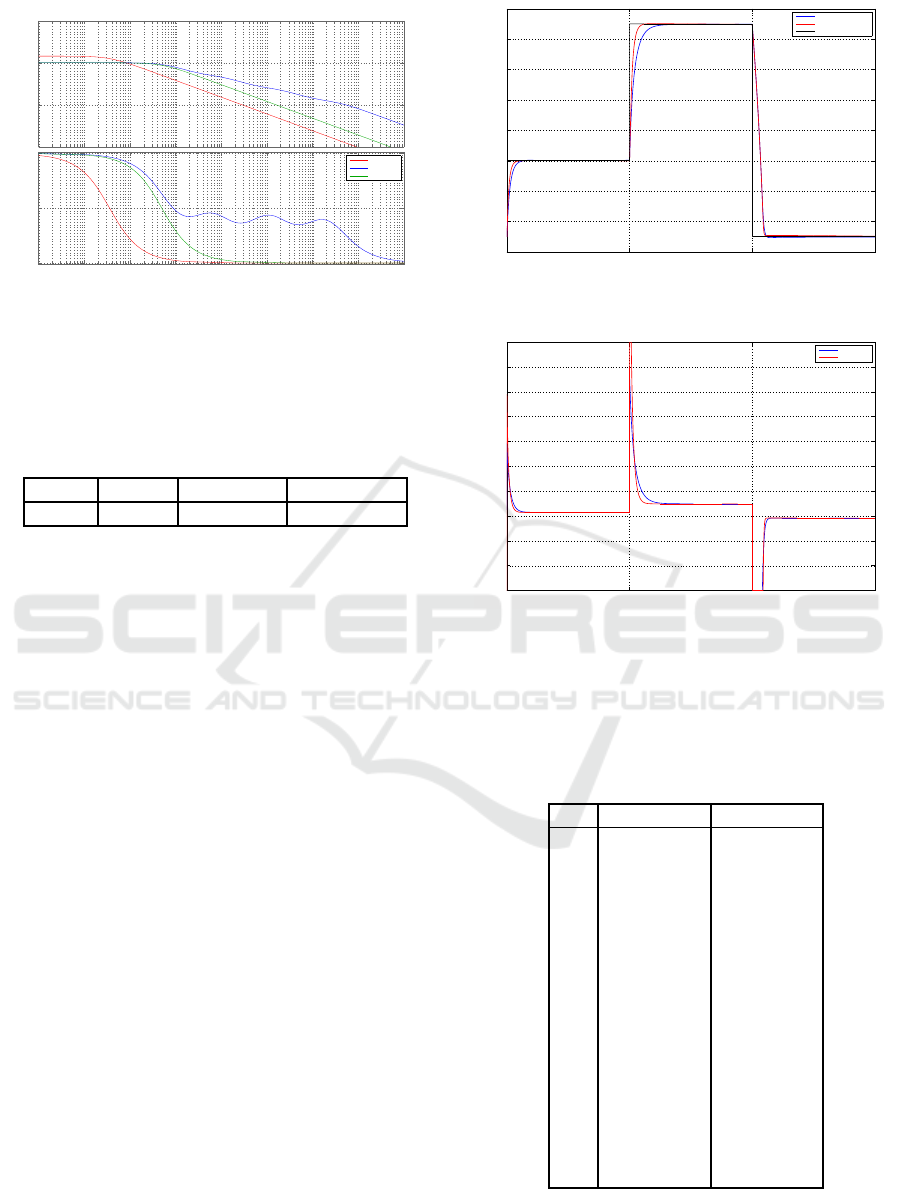
The step response of the fractional order refer-
ence model is compared with that of the integer order
model and with the open loop system step response in
Figure 3.
Figure 4 illustrates the bode plot of the open loop
system, of the integer order reference model, and the
fractional order reference model.
0 500 1000 1500 2000 2500
0
0.5
1
1.5
2
2.5
Step Response
Time (seconds)
Amplitude
Figure 3: Open loop step response of the tank system (red),
step response of the integer order reference model (green),
step response of the fractional order reference model (blue).
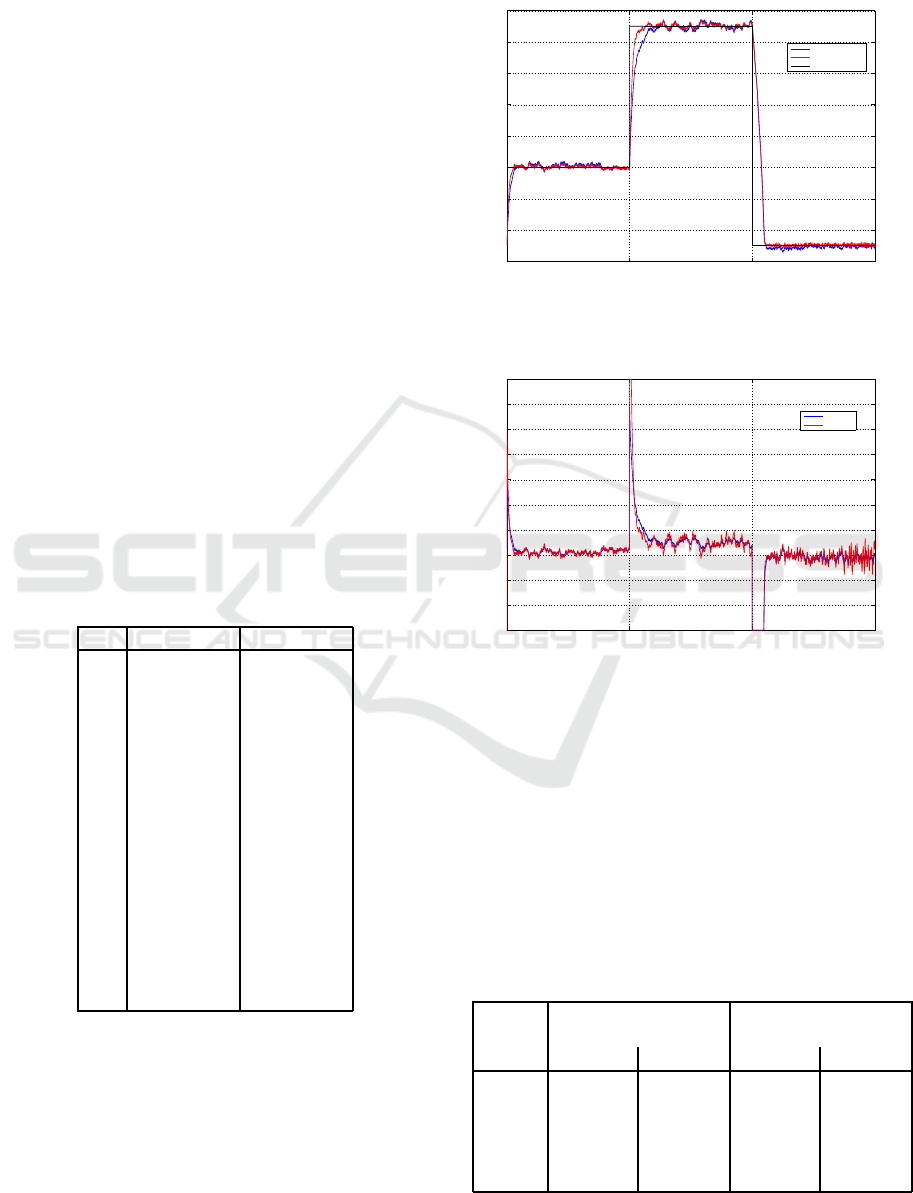
From Figure 3, we clearly see that the fractional
order model is faster than the integer order model,
which is confirmed also in Figure 4, where we see
that the fractional reference model has the largest pass
band.
In order to test the effectiveness and the performances
Conical Tank Level Supervision using a Fractional Order Model Reference Adaptive Control Strategy
217
−100
−50
0
50
Magnitude (dB)
10
−4
10
−3
10
−2
10
−1
10
0
10
1
10
2
10
3
10
4
−90
−45
0
Phase (deg)
Bode Diagram
Frequency (rad/s)
G_sys
Gm_frac
Gm_entier
Figure 4: Bode plot of G (red), of G
m
(red), and of G
mf
(blue).
of each controller (MRAC and FO-MRAC), a stan-
dard reference signal u
r
(t) is applied, consisting of
steps with different amplitudes described in table 2.
Table 2: Reference signal.
t (sec) [0 500] [500 1000] [1000 1500]
r(t) 20 29 15
Also, to evaluate and compare the performances
of each control method, we choose the performance
index given by the sum of the absolute error (SAE) de-
fined in the expression (26), and the sum of the square
input (SSI) defined in (27):
J
e
=
N
∑
k=0
|e(k∆)| (26)
J
u
=
N
∑
k=0
u(k∆)
2
(27)
where N is the samples number, e(k∆) = y(k∆) −
r(k∆).
5.1 Study in the Ideal Case (Without
Disturbances)
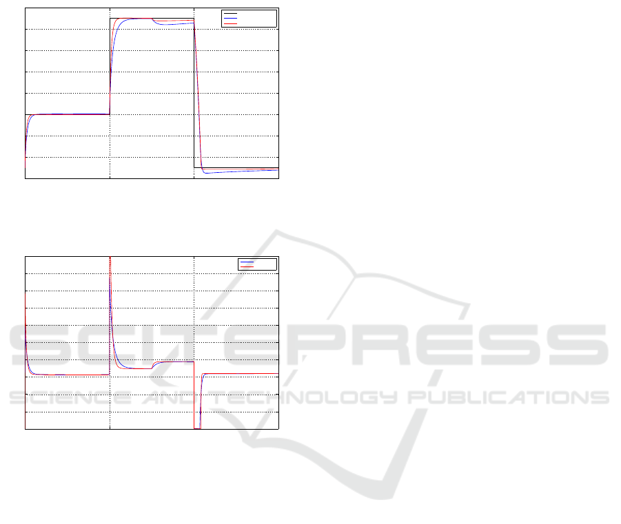
Respectively, the real output of the system and the
control signal of the classical MRAC and the FO-
MRAC are shown in Figure 5 and Figure 6.
From obtained results, we remark that the output
of the system follows the referential signal, even the
sudden change of the set point signal.
Better results are obtained when using the FO-MRAC
method, where we have the lowest cost function of
error, whereas the MRAC strategy presents the lowest
energy consumption by the control signal. The sys-
tem is faster and more precise with the FO-MRAC
strategy.
In order to study the influence of the fractional order
0 500 1000 1500
14
16
18
20
22
24
26
28
30
Time (sec)
System output
Classical MRAC
FO−MRAC (m=1.1)
Setpoint signal
Figure 5: The system response with classical MRAC and
with FO-MRAC (m = 1.1).
0 500 1000 1500
0
10
20
30
40
50
60
70
80
90
100
Time (sec)
Error signal
MRAC
FO−MRAC
Figure 6: The control signal of the classical MRAC and the
FO-MRAC (m = 1.1).
m value on the performance of the control system, we
vary its value from 0.1 to 1.5; the results are grouped
in the following Table 3.
Table 3: Cost functions Versus the fractional order m.
m J
e
J
u
0.1 5.6025 10
3
1.6313 10
7
0.2 5.6011 10
3
1.6313 10
7
0.3 5.5988 10
3
1.6313 10
7
0.4 5.5948 10
3
1.6314 10
7
0.5 5.5879 10
3
1.6315 10
7
0.6 5.5758 10
3
1.6318 10
7
0.7 5.5550 10
3
1.6322 10
7
0.8 5.5207 10
3
1.6331 10
7
0.9 5.4667 10
3
1.6346 10
7
1 5.6484 10
3
1.6096 10
7
1.1 5.3649 10
3
1.6424 10
7
1.2 5.5223 10
3
1.6332 10
7
1.3 5.4757 10
3
1.6348 10
7
1.4 5.4264 10
3
1.6377 10
7
1.5 5.4376 10
3
1.6369 10
7
From the results, the minimum cost of the error is
obtained for m = 1.1, where the control energy con-
ICINCO 2018 - 15th International Conference on Informatics in Control, Automation and Robotics
218
sumption is the greatest. The error cost function is
better for FO-MRAC whereas the criterion J
u
is better
for integer order MRAC, which means that the frac-
tional order MRAC improves the reference tracking
by mean of a greater input energy effort.
From the Table 3, there exists a trade off between
the control energy consumption and the tracking error
cost. The FO-MRAC strategy allows the resolution of
this trade off by choosing the proper m value.
It is also worthy to notice that the adaptation gain γ is
very small for all fractional orders m (less than 10
−6
)
comparatively to the integer order MRAC (γ = 0.01)
which improves the relative stability of the adaptive
control system.
5.2 Study in the Presence of
Measurement Noises
In order to test the robustness of these controllers in
the case where the measurement is tainted with noise,
we have injected a noise to the output (random signal)
of zero average and standard deviation equal to 0.03.
We study the influence of the fractional order m value
on the performance of the FO-MRAC system in pres-
ence of measurement noise by varying its value from
0.1 to 1.5, the results are grouped in Table 4.
Table 4: Cost functions Versus the fractional order m in
presence of noises.
m J
e
J
u
0.1 7.0855 10
3
1.6168 10
7
0.2 7.0839 10
3
1.6168 10
7
0.3 7.0812 10
3
1.6168 10
7
0.4 7.0763 10
3
1.6169 10
7
0.5 7.0673 10
3
1.6170 10
7
0.6 7.0509 10
3
1.6173 10
7
0.7 7.0215 10
3
1.6177 10
7
0.8 6.9698 10
3
1.6185 10
7
0.9 6.8811 10
3
1.6201 10
7
1 8.1872 10
3
1.5961 10
7
1.1 6.5166 10
3
1.6305 10
7
1.2 6.9527 10
3
1.6186 10
7
1.3 6.8560 10
3
1.6202 10
7
1.4 6.6940 10
3
1.6235 10
7
1.5 6.7269 10
3
1.6226 10
7
From Table 4, we see that the FO-MRAC is more
robust against noise than the classical MRAC strat-
egy, for the reason that with FO-MRAC, we obtain
always the lowest error cost and that for any value of
the fractional order of integration m. The lowest error
cost is obtained for m = 1.1.
Figure 7 and Figure 8 illustrate respectively the sys-
tem output and the control signal for the two applied
strategies.
0 500 1000 1500
14
16
18
20
22
24
26
28
30
Time (sec)
System output
Classical MRAC
FO−MRAC (m=1.1)
Setpoint signal
Figure 7: The system response with classical MRAC and
with FO-MRAC (m = 1.1) in presence of measurement
noises.
0 500 1000 1500
0
10
20
30
40
50
60
70
80
90
100
Time (sec)
Control signal
MRAC
FO−MRAC
Figure 8: The control signal of the classical MRAC and the
FO-MRAC (m = 1.1) in presence of measurement noises.
5.3 Study in Case of Model Parametric
Variations
No let us test the robustness of the proposed control
law with respect to model parametric variations. We
consider a set of variation on the parameter values
in equation (23) from the instant 1500 sec. Results
obtained with the classical MRAC and with the FO-
MRAC strategy are exposed in Table 5.
Table 5: Cost functions Versus the parameter variation rate.
Param Classical FO-MRAC
var. MRAC m = 1.1
% J
e
J
u
J
e
J
u
05 7.0710
3
1.65 10
7
5.1310
3
1.6710
7
10 7.5510
3
1.68 10
7
5.2810
3
1.7210
7
20 8.6110
3
1.76 10
7
5.6710
3
1.79 10
7
40 1.0710
4
1.92 10
7
8.4010
3
1.94 10
7
60 1.2310
4
2.10 10
7
1.0010
4
2.12 10
7
Conical Tank Level Supervision using a Fractional Order Model Reference Adaptive Control Strategy
219
The system responses for the two control strate-
gies applied in case of 20% parameter variation and
the control signal of the classical MRAC and the FO-
MRAC controllers are exposed in Figure 9 and Fig-
ure 10.
0 500 1000 1500
14
16
18
20
22
24
26
28
30
Time (sec)
System output
set point signal
Classical MRAC
FO−MRAC (m=1.1)
Figure 9: The system response with classical MRAC and
with FO-MRAC (m = 1.1) in presence of measurement
noises.
0 500 1000 1500
0
10
20
30
40
50
60
70
80
90
100
Time (sec)
Control signal
MRAC
FO−MRAC
Figure 10: The control signal of the classical MRAC and the
FO-MRAC (m = 1.1) in presence of measurement noises.
From the simulation results, we see that w the sys-
tem is affected by the change of parameter value at
the instant of 1500 sec, after that we observe that the
system tries to follow the consign signal, and at the
end maintains the desired performance. However, it
is also remarkable that with an FO-MRAC strategy,
the error signal has the lower amplitude.
From the Table 5, we see that the FO-MRAC has al-
ways the lowest error cost, even for sudden parameter
variations. So, we conclude that the FO-MRAC is
much more robust than the classical MRAC.
6 CONCLUSIONS
A fractional order model reference adaptive control
has been designed in order to command a conical tank
level with nonlinear dynamics. The reference model
is set to be a fractional model system approximated by
rational transfer function using the singularity func-
tion approach; also a fractional order parameter adap-
tation law is used to update the controller parameters.
Simulation results illustrate the effectiveness of the
proposed control scheme and confirm its robustness
and especially in the presence of measurement noises
and parametric variations.
REFERENCES
Bourouba, B., Ladaci, S., and Chaabi, A. (2018). Re-
duced order model approximation of fractional order
systems using differential evolution algorithm. Jour-
nal of Control, Automation and Electrical Systems,
29(1):32–43.
Charef, A., Sun, H. H., Tsao, Y., and Onaral, B. (1992).
Fractal system as represented by singularity function.
IEEE Transactions on Automatic Control, 37:1465–
1470.
Chen, Y., Cheng, S., Wei, Y., and Wang, Y. (2016). Indirect
model reference adaptive control for a class of linear
fractional order systems. In American Control Con-
ference (ACC), Boston, MA, USA. IEEE.
Deghboudj, I. and Ladaci, S. (2017). Fractional order
model predictive control of conical tank level. In
on Automatic control, Telecommunication and Signals
(ICATS17), Annaba, Algeria, 11–12 December, pages
1–6. IEEE.
El-sayed, A. and Gaafar, F. (2003). Fractional calculus and
some intermediate physical processes. Applied Math-
ematics and Computation, 144:117–126.
Jauregui, C., Duarte-Mermoud, M., Orostica, R., Travieso-
Torres, J., and Beytia, O. (2016). Conical tank level
control using fractional order pid controllers: a sim-
ulated and experimental study. Control Theory Tech,
14(4):369–384.
Ladaci, S. and Bensafia, Y. (2016). Indirect fractional or-
der pole assignment based adaptive control. Engineer-
ing Science and Technology, an International Journal,
19(1):518–530.
Ladaci, S. and Charef, A. (2003). Mit adaptive rule with
fractional integration. In CESA 2003IMACS Multicon-
ference Computational Engineering in Systems Appli-
cations, Lille, France.
Ladaci, S. and Charef, A. (2006). On fractional adaptive
control. Nonlinear Dynamics, 43(4):365–378.
Ladaci, S. and Charef, A. (2012). Fractional adaptive con-
trol: A survey. In Classification and Application
of Fractals: New Research Edited by:E.W. Mitchell
and S.R. Murray., pages 261–275. NOVA Publishers,
USA.
Ladaci, S., Loiseau, J., and Charef, A. (2008). Fractional or-
der adaptive high gain controllers for a class of linear
systems. Communications in nonlinear science and
numerical simulations, 13(4):707–714.
Ma, J., Yao, Y., and Liu, D. (2009). Fractional order model
reference adaptive control for hydraulic driven flight
ICINCO 2018 - 15th International Conference on Informatics in Control, Automation and Robotics
220

motion simulator. In SSST 2009, 41st Southeasten
Symposium on System Theory. Tullahoma, TN, USA.
IEEE.
Mathieu, B., Melchior, P., Outsaloup, A., and Ceyral, C.
(2003). Fractional differentiation for edge detection.
Signal Processing, 83:2421–2432.
Oldham, K. and Spanier, J. (1974). The fractional Calculus.
Academic Press, New York.
Outsaloup, A. (1991). La commande CRONE (in French).
Herm`es, Paris.
Outsaloup, A. (1995). La d´erivation non enti`ere (in French).
Herm`es, Paris.
Podlubny, I. (1999). Fractional order systems and pi
λ
d
µ
controllers. IEEE Transactions on Automatic Control,
44(1):208–214.
Vinagre, B., Petras, I., Podlubny, I., and Chen, Y. (2002).
Using fractional order adjustment rules and fractional
order reference models in model-reference adaptive
control. Nonlinear Dynamics, 29:269–279.
Warier, S. and Venkatesh, S. (2012). Design of controllers
based on mpc for a conical tank system. In Interna-
tional Conference On Advances in Engineering, Sci-
ence and Management, Tamil Nadu, India, pages 309–
313. IEEE.
Conical Tank Level Supervision using a Fractional Order Model Reference Adaptive Control Strategy
221
